Search

Each research flight of the King Air required: i) selection of a scientific mission based on the expected weather conditions, ii) determination of the flight’s takeoff and landing times and flight plan, iii) requests for any required radiosonde support with launch times and locations, and iv) the ability to make changes in this plan as the flight developed. Since the project involved the Wyoming flight crew and universities in four different cities, special methods of communication were needed to accomplish these requirements. Different approaches were used prior to, during, and after a daily noon planning meeting.

The process began with a forecast. Due to time spent on other aspects of the project leading up to the start of operations on 4 NOV (e.g. ground equipment installation), the first meeting with prospective student forecasters did not occur until 31 OCT. It had previously been decided that Millersville University students would develop the forecasts and host the video conference. The call for forecasters was distributed to all Millersville meteorology students with a requirement of one-semester participation in the Campus Weather Service, which would provide students with the practical experience and knowledge of products useful in creating forecasts.

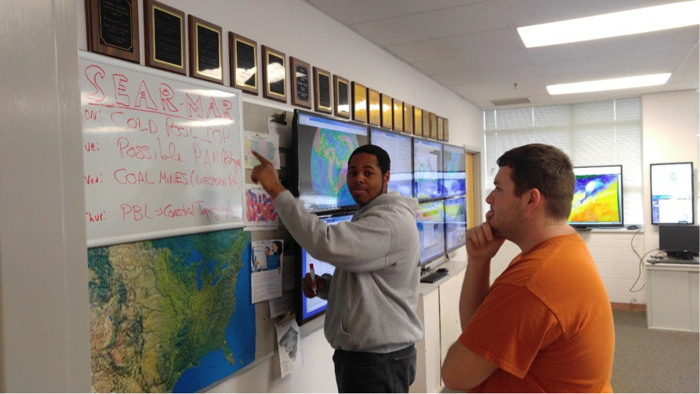
To further leverage the Campus Weather Service, SEAR-MAR students prepared a 5-day forecast each day after the normal 0730 LST weather briefing used to develop a local forecast for Millersville University. With guidance from faculty, the forecasters wrote a summary of the expected weather conditions each day and identified the most favorable scientific mission based on a description of the relevant flight plan and approximate flight times. This was the first document distributed to an e-mail list, which included lead scientists, research associates, the Wyoming crew, and over 100 students at the four institutions. The one-line summaries were also kept on a whiteboard in the Millersville University Weather Information Center (MUWIC) as shown in Figure 5.

On the day before a potential flight, an additional forecast was prepared one hour before the daily planning meeting to confirm the best mission and add additional information from higher resolution models. This was also distributed by e-mail to the same listserv. While the forecasts were intended to be guides to research mission selection, and were occasionally superseded by other participants’ analysis, they ended up having great weight in determining the flight was chosen, so that the students involved in the forecasting were also effectively gaining experience field experiment operations.

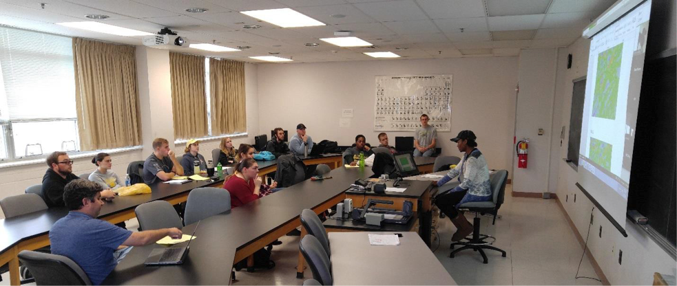
The most important communication between partners was the planning meeting, which was held at noon every day of the project until the flight hours were expended. This meeting was used to formally declare the mission and its parameters, including when radiosondes would be launched and from which site. Other announcements of relevance to the project could also be made. While a classroom on the Millersville campus allowed many students from that campus to attend (Fig. 6), any participant could easily join by phone or video conference. The latter made for a more familiar meeting situation and could even be used to provide live weather updates during IOPs. It was also beneficial that the Wyoming crew could join from the airport in close proximity to takeoff and landing times.

For subsequent changes to the mission plan there was first a pre-flight forecast update, which was prepared by that day’s student forecasters and delivered by one of them using video conferencing three hours before the declared takeoff time. This allowed observations and the highest-resolution model runs to be incorporated into the outlook, while also allowing enough time to train those students who were to fly that day. While the start time could not be moved forward after the pre-flight update, it could be pushed back for more favorable conditions or to accommodate slight modifications to the flight plan.

After the flight was airborne, communication was still possible using chat software available on the King Air and to any interested participants on the ground. An important ground station was MUWIC where there was always one or more people following the progress of the mission. If data from early legs was not as expected, mission scientists on the ground could suggest or approve changes to improve the results, such as shifting legs laterally or to a higher altitude. On occasion, chat was also used at Millersville’s ground site if that was involved in the mission, or to communicate with the mobile radiosonde crew.

Mission identification in this section follows that employed by the UWKA staff, and found at, http://flights.uwyo.edu/projects/searmar17/.

• RF01 - Cold Air Damming
• RF02 - Fine Structure of Cold Fronts
• RF05, RF06, RF13a, RF13b - Methane
• RF07 - Mountain Lee Waves
• RF08 - Cold Pool and Northerly Low-Level Jet
• RF09 and RF12 - Ocean-Bay-Land PBL Height Variability
• RF10 - Static Pressure Defect
• RF11 and RF14 - PAM

On 6 November 2017, a mission was flown (RF02) in support of the first science objective to investigate the fine structure of cold fronts. The UWKA departed KLNS at 1400 UTC and returned at 1753 UTC. The mission was to ascend to and maintain constant altitude at 1500 m AGL). Fig. 7 shows the UWKA flight track created using Google Earth.®

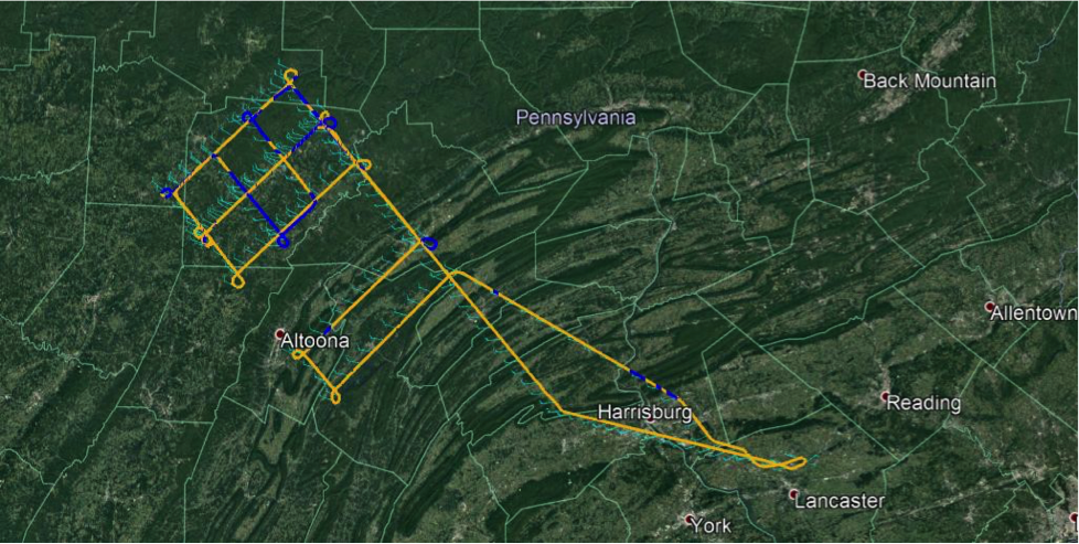
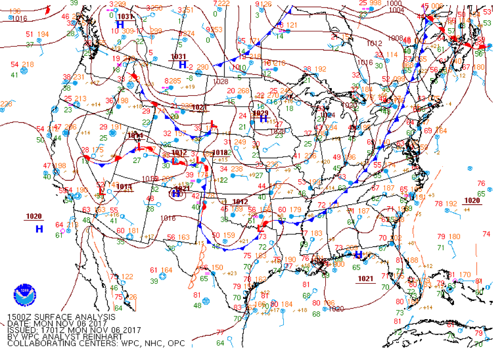
The UWKA transited first to the Allegheny Plateau, where a series off lawnmower tracks were flown in the vicinity of the analyzed surface front in Figure 8. The lawnmower pattern was selected to investigate the terrain-induced influence on frontal ebb and surge, discrete propagation of fronts, frontal width, and narrow cold-frontal rainband passage.

That cold front moved quickly to the southeast during the mission, being located near Philadelphia, PA by 1800 UTC 5 November 2017 WPC surface analysis (not shown). An attempt was made to sample the cold front after it moved from the Allegheny Plateau to the convoluted ridge and valley system southwest of State College, PA. Hence, the UWKA flew a second truncated southern lawnmower pattern before returning to KLNS.

Radiosondes were launched in support of the RF02 mission by PSU at University Park, PA at 1200 UTC, 1500 UTC, and 1800 UTC (all 6 November 2017). Radiosondes were also launched by MU at 1800 UTC, 2100 UTC, (both on 6 November 2017) and at 00000 UTC on 7 November 2017.

As of the time of this writing, data from the UWKA for this mission as not been analyzed in detail. Erin Jones, senior MU meteorology major, Honors College Scholar, and Hollings Scholar, is using SEAR-MAR data obtained during this science mission for her Honors thesis, entitled the “Impact of local radiosonde observations in high-resolution WRF simulations.”

Another mission with high student involvement was based on a larger research project proposed by a group of Millersville students independent of SEAR-MAR or any meteorology course. Their goal over a two-year period is to perform the research, present the preliminary results at a series of conferences (the first being the annual Made in Millersville student conference; Dellandre et al. 2018), and ultimately author a journal article. The work involves a case study comparison of two cold air damming (CAD) events, and with the availability of the UWKA the second event could be supported by a unique dataset (see RF01 in Table 1).

These students made an initial attempt to design a flight path over the valleys near Altoona, PA, the site of a significant historical CAD event. However, due to the King Air’s minimum altitude, these tracks turned out to be beneath the local crestline of the Appalachians. Therefore, the study area was shifted southward to the Cumberland Valley and downwind of the Blue Ridge Mountains (Fig. 10) with two flight altitudes and slow climbs and descents in between. There were also three missed approaches planned at small airports in Carrol County, MD and Franklin County, PA. Three MU students flew on the UWKA during this mission.

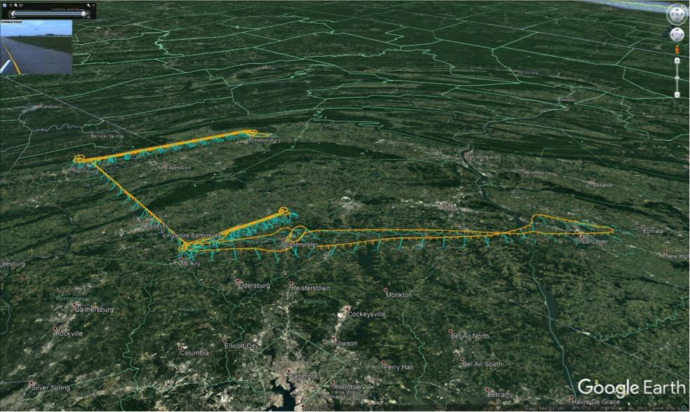
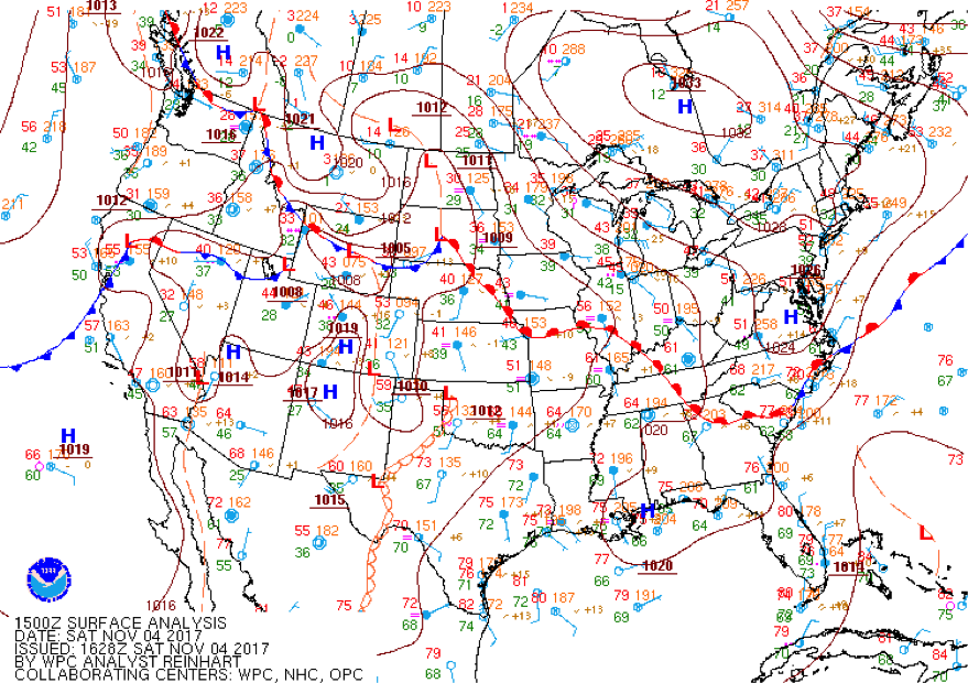
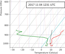
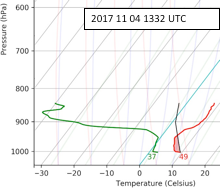
The ideal synoptic conditions occurred on the first day of the deployment (4 Nov) with a closed high forecast over the Ontario-Manitoba border and ridging isobars extending southward to Virginia (Fig. 11). While daylight conditions were required to fly the minimum altitudes, the mission was otherwise scheduled as early as possible to minimize the amount of heating and surface erosion of the cold air, so that takeoff was at 12 UTC (08 LST).

The rest of the student research team provided additional ground support by launching two Windsonds along the flight path. They first traveled to the Sharpsburg, MD area at 1230 UTC to obtain a sounding in the Cumberland Valley directly under the ferry leg. This was timed to coincide with the King Air’s overpass by communicating with students in Millersville’s Weather Center who were following the flight on NCAR Mission Coordinator. Moving north, students launched a second balloon. Both sondes were recovered after the second launch. To capture additional horizontal variation in the vertical structure, radiosondes were also used from the Millersville base site at 1230 UTC and by PSU at Bedford, PA at 1130 UTC.

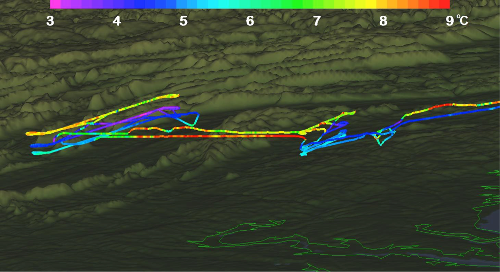
During the first missed approach and mountain parallel flight legs, it was found that temperature was higher nearer to the surface. However, as the King Air was ferrying westward, the plane was forced to climb to 4000’ to pass ATC at Frederick, MD. At this level, the warmer temperatures of the inversion were discovered. After discussion among the flight team and with participants in the Weather Center, it was agreed to add an additional flight level at a higher elevation along both sets of ridges. This new altitude and the one beneath it were used to map out the horizontal structure of the inversion, which is shown in Fig. 12. Moreover, the students reported visually observing fanning smokestack plumes during the flight. The inversion was also captured in all of the morning radiosonde launches. While the earlier soundings from Bedford and Sharpsburg, MD (Fig. 4a) have second surface-based inversions, the later profile from Waynesboro, PA (Fig. 4b) had the same decreasing temperatures seen in the King Air data. On returning from their trip, students made particular note of this dramatic difference in surface temperature between the two launch locations. While the extra hour of solar heating would have an obvious impact, it is also possible this is due to horizontal variations between up- and down-valley locations, as the King Air observed horizontal temperature variations along its valley legs.

After the passage of a cold front, the Appalachians often experience an extended period of strong flow with a westerly and/or northerly component. In cooler, more stable air this results in the formation of trapped lee waves with trains that may propagate across the mid-Atlantic Piedmont and through the SEAR-MAR domain. Since the mountains have a sharp clockwise bend in the study area, both eastward and southward traveling waves can be triggered, and there is a possibility of interference between the two.

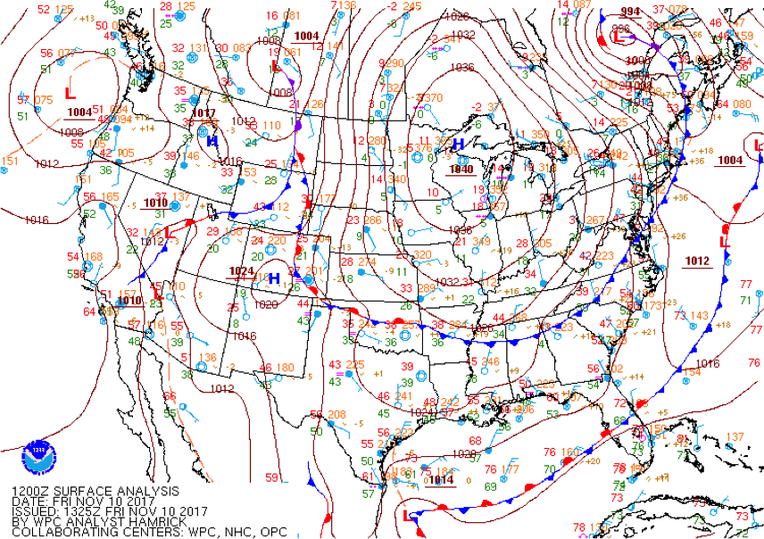
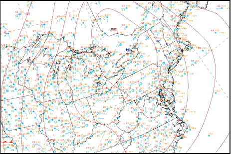
Forecast teams identified 10 Nov, after an overnight cold front passage and ahead of an advancing 1040 hPa high pressure system (Fig. 14), as an ideal mountain wave day. Short-term model guidance suggested a midday transition from wave trains to convective cloud streets, so takeoff was scheduled for 1430 UTC.

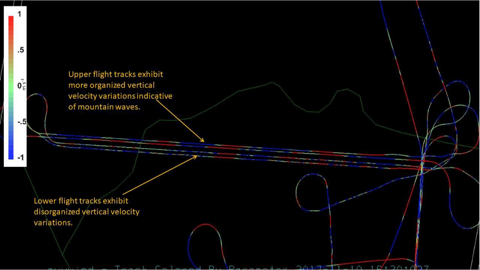
To study this phenomenon, a flight path was developed that included four vertically-stacked levels in both an N-S direction and an E-W direction (Fig. 15). Between these two stacks, in the area NE of Gettysburg, PA, a sequence of ascending legs crisscrossing the line of inflection through the Appalachians was planned, followed by a set of similar descending legs.

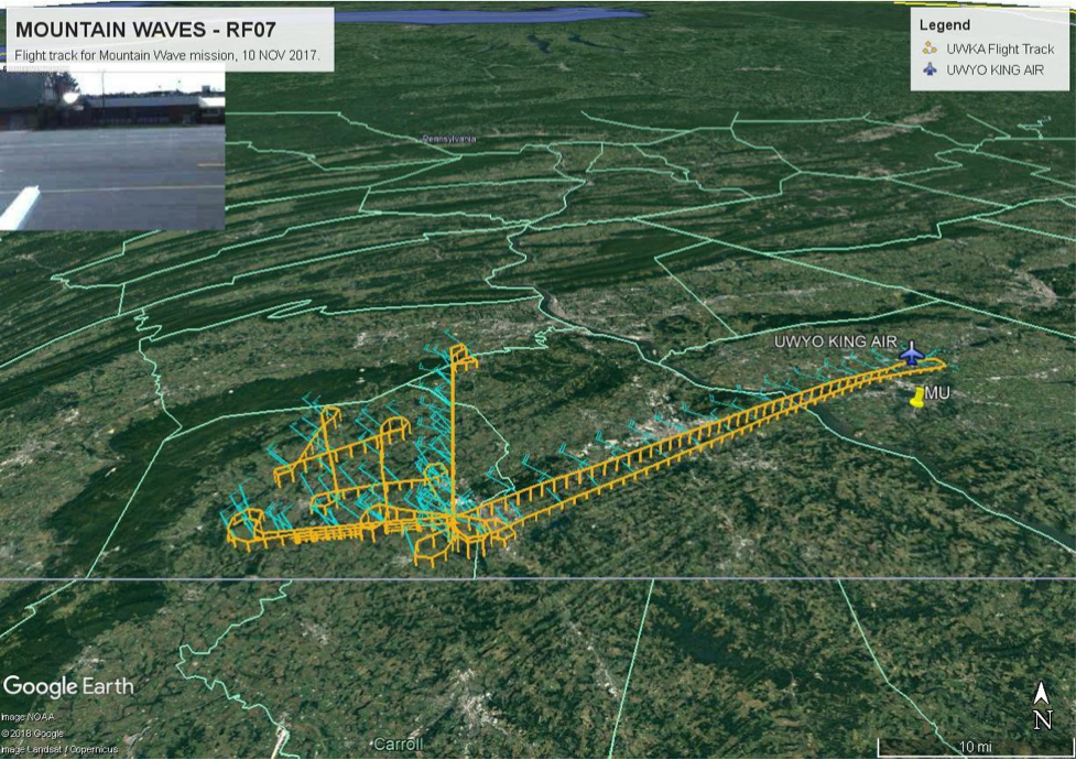
The N-S stacks had a well-defined wave structure at 6250’ AGL, but the lower three legs were found to all be within the turbulent boundary layer. For this reason, the flight plan was changed so that after the ascending zigzag, the return pattern was made at a constant 6250’ elevation. Then, one of the lower E-W legs was replaced by a higher one at 7750’ resulting in additional mountain wave transits.

Figure 16 is from a student presentation showing the inflight vertical velocities for the entire track. There are obvious differences between the irregular fluctuations in the lower transects and the smoother, periodic undulations along the transects at higher altitudes where the mountain waves reside.

The Cold Pool experiment aimed to characterize the lowest levels of the stable boundary layer across valleys of varying widths to understand terrain influences on cold pool development and dissipation in the Pennsylvanian Appalachian Mountains. All observational resources available to Millersville University SEAR-MAR participants were used, including the University of Wyoming King Air (UWKA) Research Aircraft, LiDAR, SoDAR, 10-meter flux tower, and radiosonde systems.

A climatological study of frontal passage types indicated that approximately two frontal systems would be observed during the active SEAR-MAR project phase. With similar frequency, high pressure centers or cold air damming signatures were expected to occur. The ideal synoptic requirements for the Cold Pool experiment included a weak surface pressure gradient, ideal radiational cooling the evening prior, and calm surface winds. Two of three conditions were met (Fig. 17): light winds existed in the Susquehanna Valley (KMDT, KLNS) but frequently ceased in the nearby valleys, including at Selinsgrove (KSEG), Altoona (KAOO), and even Muir Army Airfield (KMUI).

The Cold Pool experiment design revolved around the capabilities of the UWKA. The objective was to explore the boundary layer in a wide valley and narrow valley case. To observe below the 1,000 ft. AGL flight minimum, regional airport accessibility was a major factor in valley selection. Therefore, the Cumberland Valley (Franklin County Regional Airport (N68)) and the valley containing Bendigo Airport (74N) were chosen. The flight path is shown in Figure 18. Meanwhile, a Windsond launch team launched two radiosondes: one in an intermediate width valley (near Pine Grove, PA) and one in conjunction with the Schuylkill County Airport (KZER) missed approach.



Also, the flux tower, LiDAR and SoDAR measurements were to be used to describe the relatively flat environment to the south and east of the target valleys.

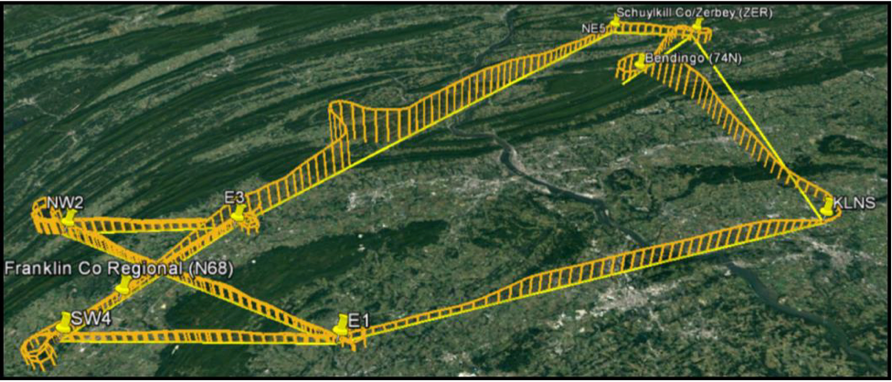
The Cumberland Valley was interrogated with the UWKA using an hourglass pattern to obtain along-valley and cross-valley characteristics at various altitudes (1,000, 1,300 and 1,600 ft. AGL). Along the entering and exiting along-valley tracks, a missed approach was included to measure the near-surface environment down to 50 ft. AGL. Upon exiting the Cumberland Valley, in transit to Bendigo, an aircraft sounding to 7,000 ft. was executed.

Two missed approaches were incorporated into exploring the Bendigo Valley. KZER presented an opportunity to measure the ridgeline near Bendigo Airport as it lies overlooking a steep slope of a similarly sized valley approximately 24 km (15 miles) to the northeast. The second Windsond launch was executed from the valley floor beneath KZER concurrently with the missed approach. From KZER, the UWKA proceeded to complete a missed approach of the narrow valley floor at Bendigo Airport followed by a sounding up to 7,000 ft. The aircraft then returned to base.

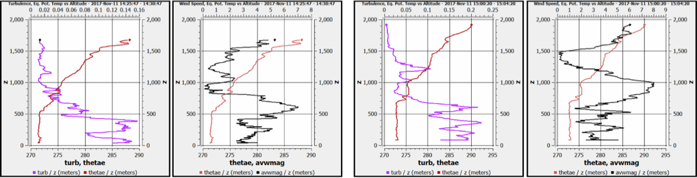
Some preliminary findings were extracted from the sounding data. The lowest portions of the boundary layer in the valley appear to have mixed by the interrogation period. However, a stable, supergeostrophic wind maximum (Fig. 19) – a northerly valley-parallel low-level jet was observed along the ridgeline above the cold pools. The structure, formation and evolution of this wind maximum has excited interest in the student group and the subject of investigation.

The planetary boundary layer (PBL) is the lowest layer of the atmosphere, encompassing surface interactions and most of the weather that affects daily life. The depth of the PBL starts at the Earth’s surface and extends anywhere from a few hundred meters to a few kilometers above the surface depending on environmental conditions. This variability in PBL height is important for air quality, atmospheric chemistry, and weather. For example, most atmospheric constituents within the PBL mix homogeneously, thus a shallow PBL confines pollutants to a small volume, whereas a deeper PBL would spread those pollutants over a larger volume thus lowering concentration and potential health risks.

While some aspects of PBL height are understood (such as the diurnal growth and decay cycle forced by solar heating), height variability over diverse surface types is not very well understood and is a valuable topic for research. In general, urban areas produce more heat and thus the PBL tends to be taller over cities. Oceans are typically cooler than land, and thus have lower PBL heights. Transitions away from these regions towards rural or coastal areas are not well characterized, in part because most PBL studies utilize fixed ground-based or radio sounding measurements that observe points, rather than spatial variation. Aircraft measurements are a great opportunity to observe this spatial variability in PBL height.

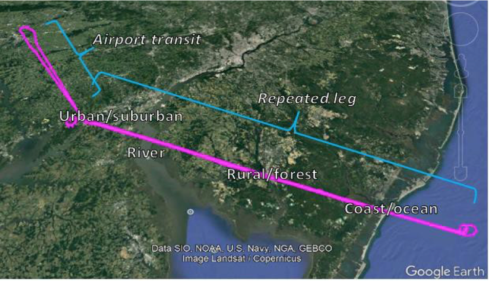
Research flight 09 (RF09) was designed to investigate the PBL height changes along a track that included urban or suburban areas, a river, rural land, forest, coast, and ocean. This track is shown in Figure 20. The flight track of interest was repeated four times to build up a robust data set. The first and fourth legs were sawtooth altitude patterns flying in and out of the PBL to measure PBL height via in situ instruments and served the purpose of characterizing the atmospheric conditions in and above the PBL. The sawtooth patterns only provide six point-measurements of PBL height along the track. Flight legs two and three provided continuous PBL height observations along the track by flying at constant altitude above the PBL, using the downward- pointing backscatter lidar onboard the aircraft to retrieve PBL heights. RF09 was conducted around 1 to 3 PM local time, when the PBL is expected to be near its maximum height for the day.

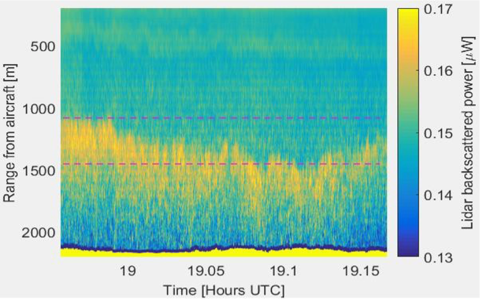
The flight was successful as planned. In situ measurements during the sawtooth pattern legs showed clear distinction between the PBL and free troposphere above it. The Wyoming Cloud Lidar (WCL) measurements during the constant altitude legs captured PBL heights with good data quality for most of the flight. A section of the third leg lidar data is shown in Figure 21; PBL height differences of 400m or more were observed along the flight path.

This analysis is still in preliminary stages. Future steps will improve data visualization and draw conclusions about PBL heights over different surface types. The impacts of the unavoidably coupled daily meteorology on this case study must also be considered. Extending beyond RF09, a similar flight path was flown for RF12 collecting PBL data shortly after sunrise. The RF12 dataset may corroborate the results of RF09, or provide new information about PBL spatial variability during the morning transition period. In the coming year, several graduate and undergraduate students will be using the data together with operational models for their research rotation work and some have expressed interest to use part of the data as a motivation in their master’s thesis study.

The PSU science objectives focused on measuring methane emissions from coal mines and a watershed where methane leaks associated with gas drilling has been identified, and measuring carbon dioxide emissions from a high density metropolitan area (Philadelphia). One project sought to quantify emissions of methane from coal mines in southwestern Pennsylvania (RF06, 09 NOV 2017). Coal mines are reported to be the largest single point sources of methane emissions in the state of Pennsylvania. Figure 22 shows a strong plume of methane emanating from the location of the coal mine.

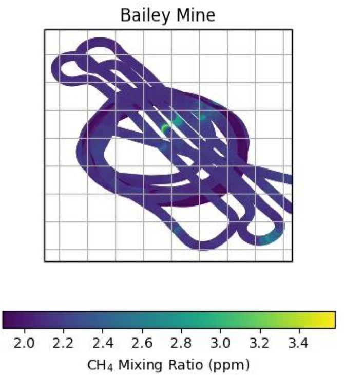
Figure 23 shows data from the same flight segments, illustrating their position with altitude. The flight levels span the entire atmospheric boundary layer (ABL) and show methane mole fractions that are elevated as much as 1.5 ppm above the upwind ABL mole fractions of about 2.1 ppm. ABL depth is about 1 km, and lower, free tropospheric mole fractions of about 1.9 ppm are observed aloft. Emission were estimates from two coal mines using a mass balance approach (Karion et al, 2015). Uncertainties in the emission rates were large due to a complex and probably polluted background in one case, and limited vertical mixing (Figure 23) in the second case. A more sophisticated analysis approach would be needed to derive a more precise estimate of emissions.

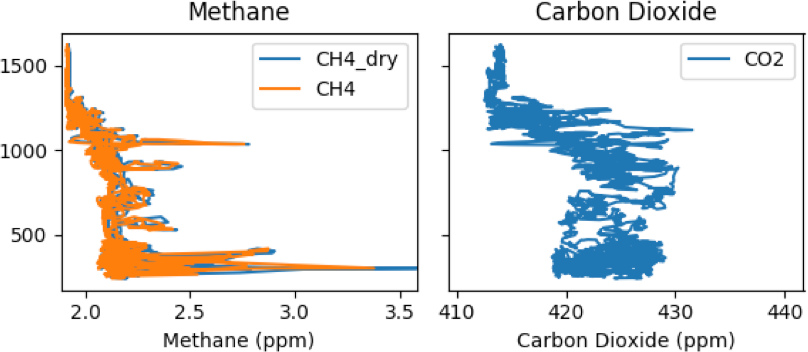
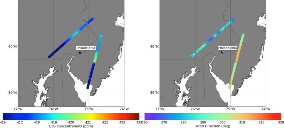
A second effort aimed to quantify carbon dioxide (CO2) emissions from Philadelphia (RF13a, RF13b). Upwind and downwind flights within the ABL (Figure 24) showed slightly elevated emissions downwind of the city, as well as heterogeneous upwind background conditions. The ABL on that day was surprisingly deep, and the flight was not high enough to locate the ABL top, leaving uncertainty concerning the depth of mixing. Emissions of CO2 were estimated (2.9x102 tons C hr-1) and were similar to the values available from a bottom-up inventory, albeit within fairly large uncertainty bounds in the airborne estimate.

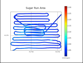
The third research flight searched for emissions from a watershed where a natural gas well is suspected to be leaking (RF05-Sugar Run-Salt Springs). Very high methane mole fractions have been measured from the ground, but no quantification of emissions into the atmosphere exists. A grid of data was collected within the ABL over the region of the suspected well failure (Figure 25). Significant, heterogeneous enhancements of 50-100 ppb of methane were observed very close to the watershed and may be associated with the emissions from the watershed. The plume structure, however, was complex and difficult to attribute to a single source location.

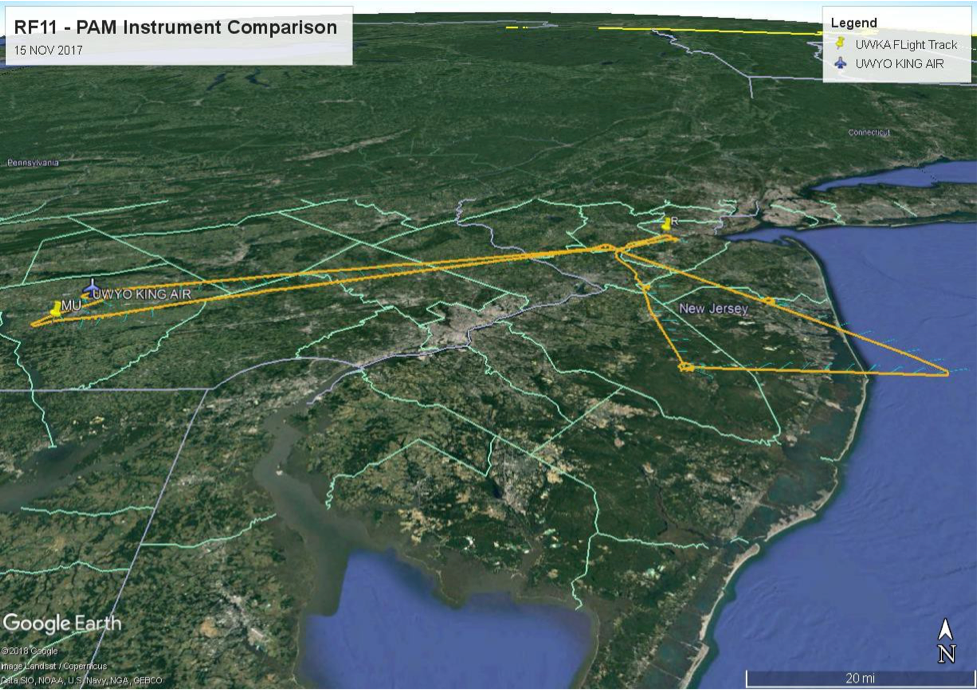
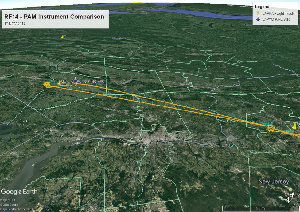
Rutgers’ involvement with the SEAR-MAR aircraft research dealt primarily with gathering information to verify the accuracy of ground-based measurements of the lower atmosphere. Specifically, the wind speed and direction measurements from a 915 MHz Wind Profiler located on Rutgers Horticulture Research Farm 3 in East Brunswick, NJ. The instrument measures wind speed/direction and virtual temperature up to about 5,000 and 1,200 meters above ground level, respectively. The research aircraft made trips to the site on two different days and provided our first ever glimpse into just how well the ground-based instrument is performing. Figure 26 shows the flight track on 15 NOV 2017, RF11, and two days later on 17 NOV 2017, RF14 was used to perform a second aircraft pass over the PAM site and the Millersville MARAF site for instrument comparison as the final flight hours were expended (Figure 27).

It is important that this instrument, first installed in 1993, is still working accurately, as the data from this profiler will not only be used in my master’s thesis which will be analyzing the longer- term trends at the site, but also because it is part of an official PAMS (Photochemical Assessment Monitoring Station) for the state of New Jersey. The profiler’s data is used by the New Jersey Department of Environmental Protection’s Air Monitoring Group to make crucial decisions about issuing air quality alerts and determining the causes of unexpected poor air quality events, so it must be accurate. As the site is situated over ‘final approach’ for Newark Liberty International Airport, launching radiosondes at the site is understandably impractical due to FAA regulations, so the aircraft flyovers were an excellent solution.

The other part of the PAMS aircraft flights were related to assessing boundary layer development over the state of New Jersey, both overland and just off the coast. The plane flew in a spiral over some set locations taking measurements to determine the boundary layer depth and dynamics.



Boundary layer measurements are an important component of many plume dispersion and behavior models, and therefore also play an important role in understanding and predicting air quality in the state. Not only that, but the comparison of the boundary layer development on land versus offshore is a valuable data set to have for future student projects.

It was also a very helpful and interesting learning experience to see and participate in the logistics behind how field campaigns operate. It’s something I don’t think very many people know about unless they’re directly involved with it. Working in the meteorology and atmospheric science field, this may not be the last field campaign I will be a part of. This campaign serving primarily as an educational and teaching deployment was a unique opportunity I feel fortunate to have been a part of. It will hopefully prepare me for future campaigns where a more basic understanding of the logistics might be assumed of the participants.

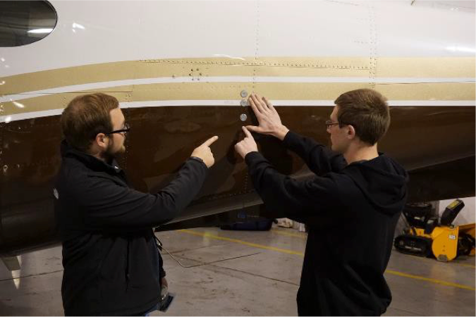
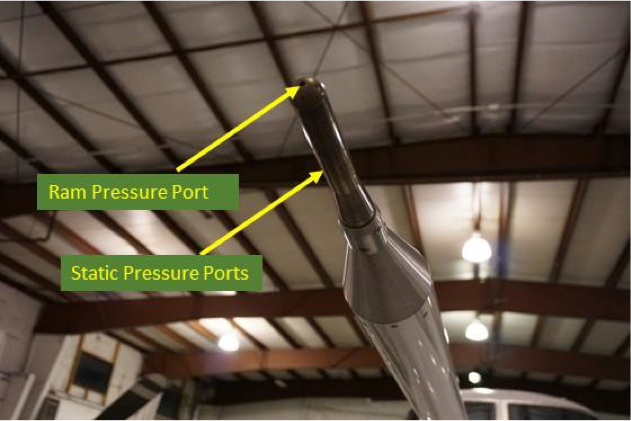
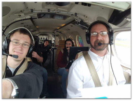
Aircraft rely on a static pressure sensor to determine airspeed and altitude from measured pressure outside the aircraft. Figure 29 shows two students identifying the location of the static pressure port on the King Air before the RF10 mission on 14 NOV 2017. The dynamic (ram) pressure data is obtained from the pressure transducer on the tip on the gust probe on the nose boom as illustrated in Fig. 30. There are static pressure ports on the nose boom as well (see Fig. 30), but they are not used in this analysis.

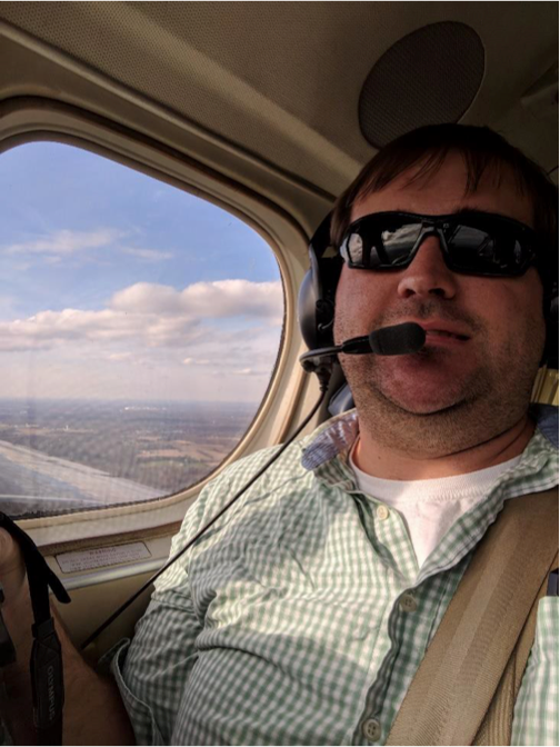
The static pressure measurements contain an inherent error or defect due to the turbulence fluctuations that impact the static pressure ports. Using data obtained during a specialized series of flight maneuvers of the UWKA, mathematical algorithms are being developed that will model the relationship between the variability in static pressure measured at the static port as a function of aircraft parameters pitch, roll, yaw, and airspeed. Statistical methods will be employed to quantify and reduce the uncertainty to a minimum. An algorithm can be used as an alternative in place of more expensive and time-consuming methods of static defect determination such as the trailing cone or tower fly-bys. The flight pattern was designed by the students, project scientists, and the UWKA crew, including the pilot (Fig. 31). The flight pattern is one of the more arduous and taxing on the crew. Students were informed before flying that in all likelihood they would experience some degree of motion sickness, and they did, but they deplaned smiling and enthusiastic.

 

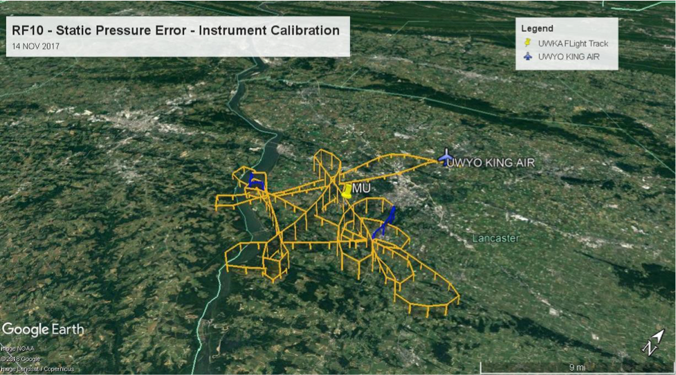
To determine fluctuations in static pressure defect, the UWKA research aircraft performed a series of variations in aircraft parameters along three spatial axes to isolate the effects of each maneuver. Pitch, yaw (heading), and airspeed were varied through a full range of aircraft motion for two minutes each at three different altitudes. The aircraft measures static pressure using two independent Rosemount 1501 High Accuracy Digital Sensing (HADS) pressure ports, two each for pilot and copilot systems, and a Weston digital vibrating cylinder pressure system. Static pressure ports are mounted aft of the wings on the fuselage (Fig. 29) and on the gust probe (Fig. 30), with each system having a static pressure port on each side of the aircraft. Data was collected at 100 Hz temporal resolution.

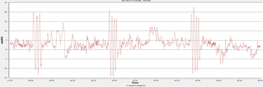
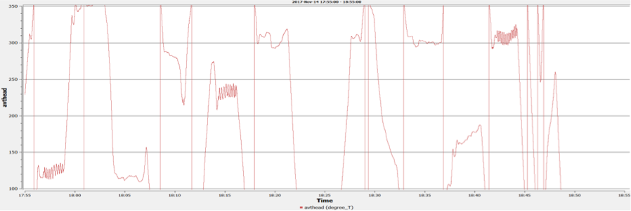
Time series of aircraft parameters pitch (Fig. 34), yaw or heading (Fig. 35), and true airspeed (Fig. 36).

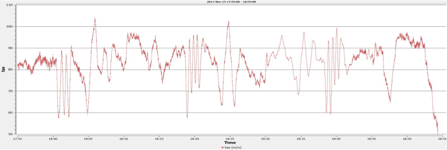
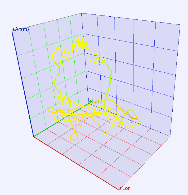
Atmospheric conditions during the flight were stable, featuring light winds and a thin stratus layer with a ceiling of 4000 ft. Each aircraft parameter was varied according to the flight plan at 1000 ft, 3000 ft, and 7000 ft AGL, and with different headings to capture variability caused by wind direction and altitude. The flight pattern followed a diamond shape with orthogonal bisecting flight legs and 270° turns at each vertex, with only minor deviations due to conflicting air traffic. The next step in this study will be to use the data collected during RF10 to develop an empirical model of the static pressure defect using a multidimensional polynomial and regress the coefficients.