A Summary of MTP Results for HIPPO-3
MJ Mahoney/JPL and Julie Haggerty/NCAR
Last Revision: March 16, 2011
We summarize on this web page, the results of the analysis of the Microwave Temperature Profiler (MTP) data obtained on the NSF/NCAR GV (NGV) during the HIPPO-3 field campaign. Its purpose is two-fold: to present the final MTP data with comments on each flight, and to discuss the excellent temperature calibration that was achieved.
Introduction
In our archived 'MP-files' we provide in the header record a comment urging users of these files to come to this web page for specfic comments on the quality of the MTP data for each of the HIPPO-3 research flights. For this reason we put the comments first in this summary. Following these comments, we provide information on how the temperature was calibrated (very successfully) for the HIPPO-3 campaign.
Comments on the HIPPO-3 MTP Final Data
The following table provides a link to a color-coded temperature curtain (CTC) for each of the HIPPO-3 test and research flights. More importantly, the table also provides a comments field where specific comments will be provided for each of the flights. Clicking on each thumbnail image will show the full-sized CTC image in a popup window, so that the image can be viewed while reading the comments. These comments are important because the rapid ascents and descents of the GV during the HIPPO campaigns degrade the quality of the MTP retrievals. On the other hand, this profiling -- as will be discussed below -- allowed very accurate temperature calibration.
First we provide an elaboration on the impact of rapid ascents and descents on the quality of the MTP retrievals. When retrievals are performed, the retrieval coefficients that we use assume that the pressure altitude is approximately constant. Clearly over an ~20 second MTP scan, this is not the case. Given a typical ascent or descent rate of ~150 m/s, 3 km are traversed in the vertical. (The actual distance is more like 2 km because not all of the 20 seconds is needed for measurements, but this is still unacceptably large.) We have tried to save as much of the ascent and descent data as possible by changing the editting threshold when it appears that the retrievals are consistent with the short level flight segments. This can be done by examining the behaviour of the tropopause or the temperature field retrievals during ascent or descent compared to those during the level flight segements.
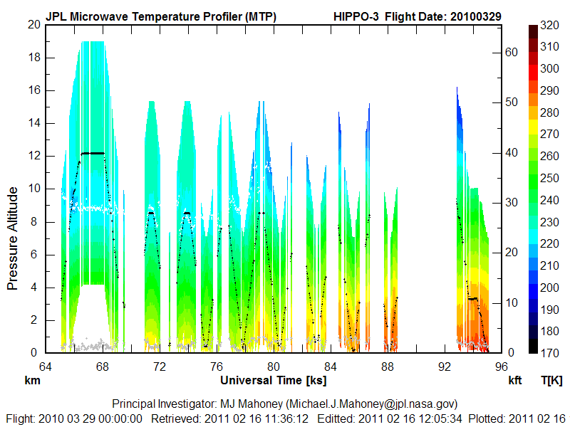
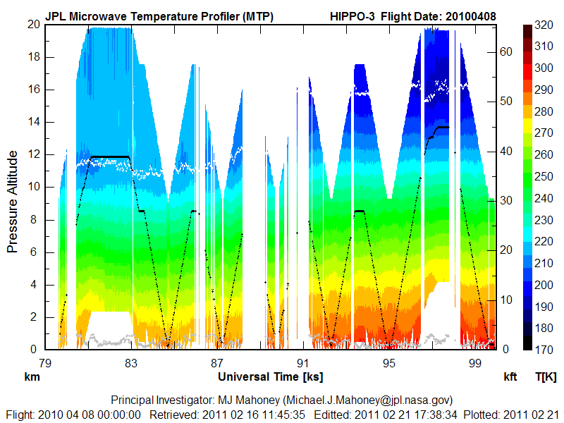
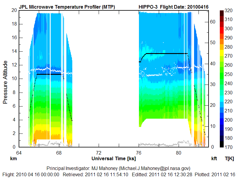
On each of the following CTC plots the x-axis it the Universal Time (UT) in kilo-seconds (ks), the left y-axis is the pressure altitude in kilometers (km), and the right y-axis is the pressure altitude in thousands of feet (kft). On the right is the color-coded temperature scale, which ranges from 170- 320 K. Also shown on each plot is the GV's altitude (black trace), the tropopause altitude (white trace), and a quality metric (gray trace at the bottom). The quality metric, which we call the MRI, ranges from 0 to 2 on the left pressure altitude scale. If the MRI is <1, we consider the retrieval to be reliable; if it is >1 the retrieval is less reliable, and users should contact use as to whether is can be used or not. With the exception of one flight (RF-02) all the MTP final data have been editted to include retrievals with the MRI<1. If this excludes a specific time period that someone is interested in, they should contact us to see whether we can salvage that time period.
For most of the flights the CTC plots (which in fact are plotted using the archived data) are restricted to ±8 km from flight level. On a few flights this was increased so that higher tropopauses could be plotted; this was the case for several tropical flights.
| CTC | Comments |
|
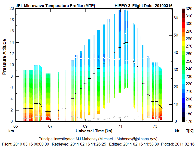
TF01 - 20100316 |
Local test flight from RMMA with RAOB comparison This short stair-step flight to make a radiosonde comparison is of good quality The rapid ascents and descents between short level flight segments have mostly been edited out |
|
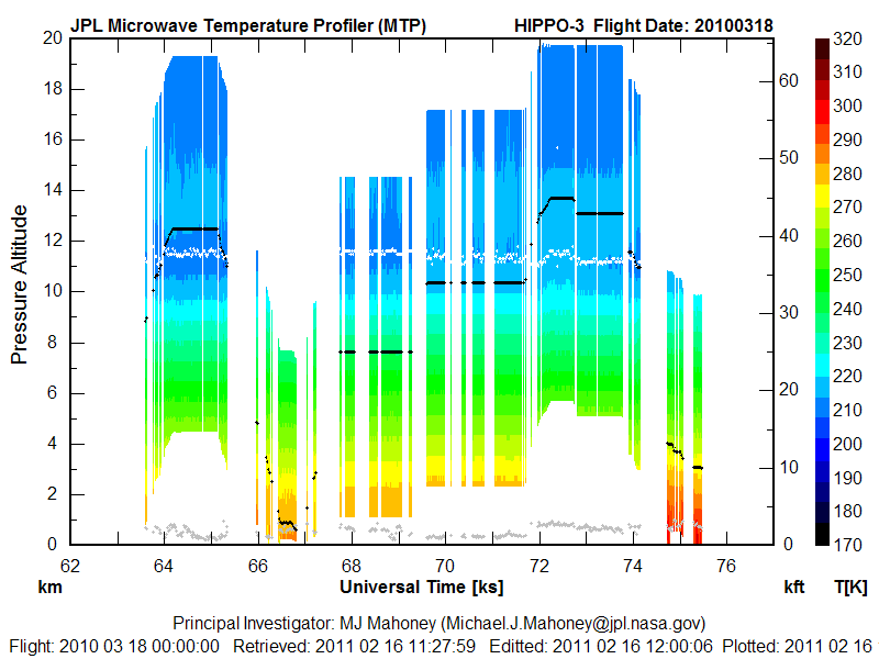
TF02 - 20100318 |
Local test flight from RMMA Most of this flight is of acceptable quality |
|
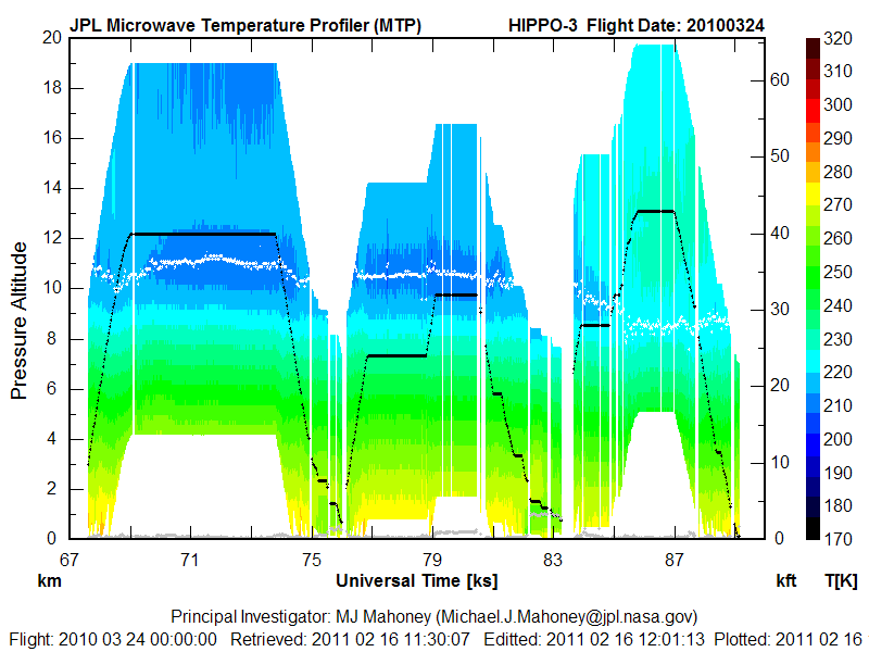
RF01 - 20100324 |
Transit flight from RMMA to Anchorage, Alaska The data for this flight looks excellent except for a short low altitude segment just before 83 ks UT |
|
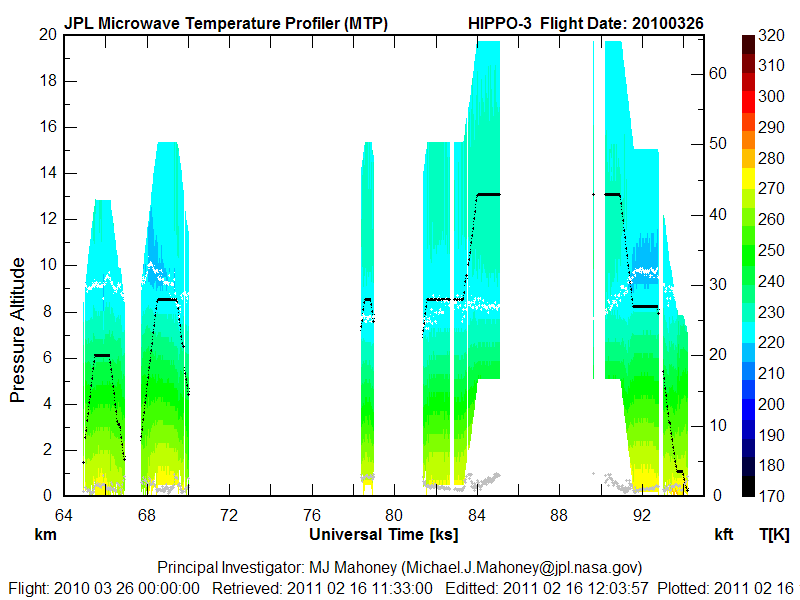
RF02 - 20100326 |
Anchorage, Alaska, to the North Pole and back This was the most challenging of all the HIPPO-3 flights to analyze. When we compared the measured brightness temperatures to those calculated from radiosondes near the GV flight track they did not match each other. This was particularly the case at low altudes leading us to believe that there was some sort of interference (but of a very different nature from what we have seen on other missions). This is particularly the case from 70-78 ks, and 85-90 ks. Use this editted data with caution! |
|
RF03 - 20100329 |
Anchorage, Alaska to Kona,Hawaii This flight is acceptable up to 88 ks when the MTP for some reason stopped tuning between the normal three frequency measurement mode; instead it was stuck on a single frequency. This prevented normal retrievals for the period from ~88-91 ks, when the instrument was rebooted. |
|
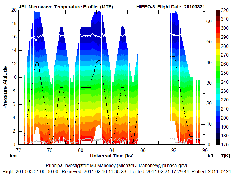
RF04 - 20100331 |
Kona,Hawaii to American Samoa This flight looks very good. The retrieval range was increased to ±10 km from flight level in order to show the tropopause. As in the previous flight the MTP got stuck on a single frequency from ~87-92 ks, so this data is lost. (We could perform a single frequency retrieval during this time period if this was important for someone. But it appears that the tropopause is consistently at ~16 km for the entire flight.) |
|
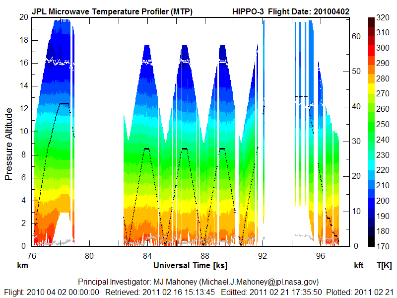
RF05 - 20100402 |
American Samoa to Christchurch, New Zealand There were two periods on this flight where the MTP frequency synthesizer collapsed to a single frequency of operation: ~79-82 ks abd ~92-94 ks. Other than that the retrievals are very good. The retrieval range was increased to ±10 km from flight level in order to show the tropopause. |
|
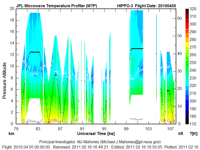
RF06 - 20100405 |
Christchurch, New Zealand to the South Pole and back Like the Anchorage to North Pole and back fligth on 20100326, this flight seemed to have some sort of strange interference. The editted data appears to be of acceptable quality although somewhat noisy. Use this data with caution. |
|
RF07 - 20100408 |
Christchurch, New Zealand to American Samoa These retrieval are a little noisy, but certainly acceptable. The tropopause behaviour from Christchurch to American Samoa appears normal, as does the low altitude temperature increase. |
|
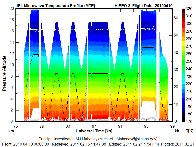
RF08 - 20100410 |
American Samoa to Kona, Hawaii We will use this flight as our "typical" performance example! The retrievals are excellent. The retrieval range was increased to ±10 km from flight level in order to show the tropopause. |
|
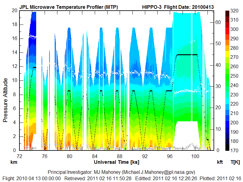
RF09 - 20100413 |
Kona, Hawaii to Anchorage, Alaska The retrievals are a little noisy, but otherwise very good. We believe that the tropopause drop near the end of the flight (~96 ks) approaching Anchorage is real. The GV likely entered the polar vortex at that time. |
|
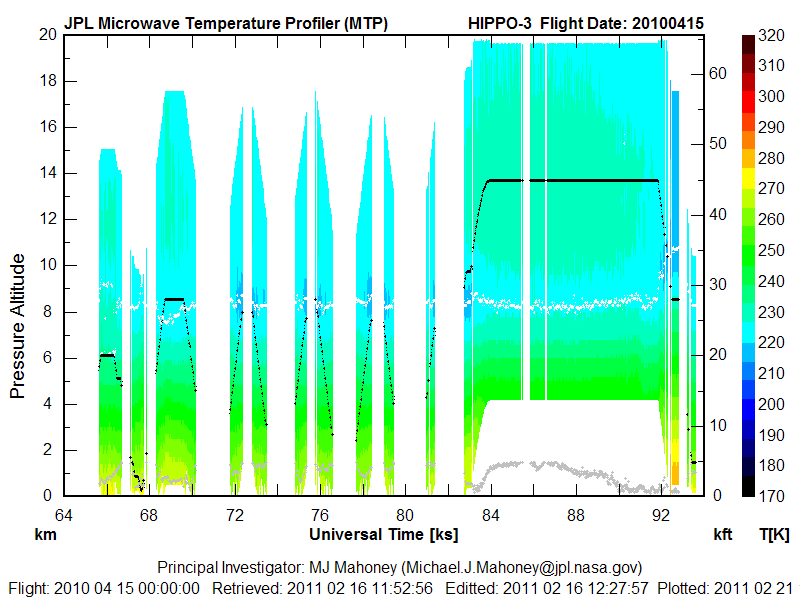
RF10 - 20100415 |
Anchorage, Alaska to North Pole and back The editted data for this flight is acceptable. Most of the editting was done during the low altitude flight segments, where there was an obvious and strong low level inversion. The retrieval coeffients did not adequately capture this inversion. If this data is important to someone, contact us and we will calculate additional retrieval coefficients to capture this inversion. The MRI threshold was increased to 1.5 salvage the data after 83 ks. |
|
RF11 - 20100416 |
Transit flight from Anchorage, Alaska to RMMA This flight is of good quality. Data is missing from 69-70 ks because the MTP was turned off for some reason. We do not know what happened. It was not a frequency collapse. |
HIPPO-3 Temperature Calibration
1) Some Background
For nearly two decades the MTP team has been refining techniques for calibrating in situ temperature measurements made aboard research aircraft using radiosondes launched near the aircraft's flight track. Initially this was done by hand, and could involve as much as a day for a single comparison because of the tedious quality control procedures that had to be implemented (such as limiting pressure altitude excursions during the comparisons, restricting allowable pitch and roll changes, and checking for radiosonde temporal and spatial variability). About a decade ago these procedures were largely automated, but the comparisons were made for the entire MTP-retrieved temperature profile at that time, not just at flight level.
Even though the MTP did not participate in the T-Rex campaign, we were asked if the MTP temperature calibration techniques could be applied to the the research and avionics temperatures measured during T-Rex so that differences in these temperatures could be resolved. During T-Rex the GV flew from RMMA to near Independence, CA, where it spent most of its flight time. In addition to the NWS soundings on transit, Leeds University frequently launched radiosondes from Independence, CA (INCA), so we had a wealth of soundings with which to do comparisons. All of the radiosondes used had an accuracy of ±0.3 K. As described on another web page, we found that both the research temperature Tres (ATRL) and the avionics temperature Tavi (AT_A) had substantial warm biases with respect to radiosondes launched near the GV flight track (Tavi - Traob = 1.21 ± 0.12, and Tres - Traob = 2.37 ± 0.12, respectively). While Tres has the largest warm bias, we also found that the Tavi warm bias is very significantly pressure altitude dependent.
This work to understand the T-Rex in situ temperatures opened the door to a new approach for doing the MTP temperature calibration. As mentioned above we had previously compared the entire retrieved temperature profile to radiosondes, not just the flight level temperature. This often required several retrieval iterations through all the flights to achieve acceptable results. It was realized that if the flight level temperature was calibrated independently of the MTP data that less work would be needed. (This is the case because previously we applied a correction to the in situ temperature measurement called OATnavCOR. Therefore, everytime OATnavCOR changed we would have to recalculate the instrument gain. If the flight level temperature is accurately calibrated from the start, then OATnavCOR is always 0.0 K, and the instrument gains do not have to be recalculated. This saves a lot of effort.)
We have continued to refine the temperature calibration techniques that we developed for T-Rex on subsequent GV campaigns. There are other web pages that describe this procedure for START-08 and HIPPO-1.
Before discussing the calibration procedure for the HIPPO-3 field campaign, we will first provide a little background. During the HIPPO field campaigns the GV was for the most part continuously profiling the troposphere (and sometimes the lower stratosphere). This was a significant concern for a number of reasons:
- First, in order to obtain good temperature profile retrievals, the MTP requires that the pressure altitude of the aircraft be relatively constant during the course of a ~20 second scan. This was blatantly not the case when the GV is behaving like an atmospheric yoyo.
- Second, related to this is the fact that we have typically averaged 3 -7 scans to beat down noise introduced by mesoscale temperature variations. Such averaging would be impossible during rapid descents and ascents.
- Third, in the past we have flatly refused to do radiosonde comparisons in the troposphere because of the high lapse rate, and therefore sensitivity to altitude excursions.
- Fourth, in order to do radiosondes comparisons, you need radiosondes. Since most of the HIPPO flights were in radiosonde sparse regions (the Arctic, Antarctic and Pacific Ocean), obtaining enough comparsions to achieve good statistics would be difficult.
- Fifth, careful consideration needs to be given to the dependence of the temperature recovery factor on Mach Number. There is no way that a constant temperature recovery factor can be used when an aircraft (an its in situ temperature probes) are profiling the atmosphere.
For these reasons our hand was forced. Normally when we do radiosonde comparisons, we do them at the time of great-circle closest approach to the radiosonde launch site. We are also careful to make sure that no one radiosonde comparsion overly weights the statistics. For example, suppose that the GV was taking off or landing at an airfield where radiosondes were launched. The "closest approach" algorithm might produce multiple times of closest approach during frequent turns. We would edit out these additional comparisons to avoid overly weighting the statistics to this site. Given the sparsity of oceanic and polar radiosondes, and the desire to have good statistics, we decided to try a new approach for the HIPPO campaigns (and other campaigns where atmospheric profiling is common). Instead of using the great-circle time of closest approach to make the comparison, we decided to do comparisons every 2 km in altitude from 2 km on up with the closest radiosonde launch site that was available. (If the closest radiosonde launch site was very distant, we had a filter that would exclude soundings beyond a specified distance threshold.) This approach would increase the number of potential comparisons by nearly an order of magnitude. But equally as important, it would allow us to assess whether any of the in situ temperature measurements had a pressure altitude dependence, which, as we remarked above, was the case for the avionics temperature during T-Rex. In addition to allowing tropospheric radiosonde comparisons, we would also be forced to abandon averaging of scans to beat down the mesoscale temperature noise, since (when profiling) the temperature change due to altitude change completely dominates any change due to mesoscale temperature variations.
2) What We Did For HIPPO-3
For HIPPO-3 there were five in situ temperature measurements that were available for radiosondes comparisons: AT_A, ATHL1, ATHL2, ATHR1, and ATHR2. (The fast response temperature ATFR was not used -- apparently because it ices up.) When we analyzed the data for HIPPO-1, we initially attempted to do a correction to the in situ temperatures as a function of pressure altitude. However, since the correction from total temperature (Tt) to static temperature (Ts) involves Mach Number squared (see this web page for more information, this equation ignores the recovery factor):
and the MTP data processing software did not use Mach Number, we needed to create a proxy for Mach Number as a function of pressure altitude Zp. We did this for a segment of a HIPPO-1 flight on 20090109, and obtained:
M2(Zp) = 0.02089 + 0.06555 Zp - 0.00122 Zp2
This approach has some inherent error however, since there is not a one-to-one correspondence between pressure altitude and Mach Number. Therefore, when dealing with the HIPPO-3 (and to be completed HIPPO-2) temperature calibrations, we decided to update the data analysis software and spreadsheets to use Mach Number squared (M2). Using Tx to represent one of the five in situ temperature measurements available for HIPPO-3, we plotted Tx-Traob versus M2, and found for the corrected temperatures (sub-script 'c'):
AT_Ac = AT_A * (1 - 0.0079 * M2) + 0.51
ATHL1c = ATHL1 * (1 + 0.0140 * M2) + 0.21
ATHL2c = ATHL2 * (1 + 0.0177 * M2) - 0.15
ATHR1c = ATHR1 * (1 + 0.0188 * M2) - 0.71
ATHR2c = ATHR2 * (1 + 0.0176 * M2) - 0.41
The Mach Number corrections for these corrected temperature measurements are important. For example the maximum value of Mach Number squared when we made radiosonde comparisons was 0.65. If we assume a nominal temperature of 200 K at this Mach Number then the corrections in these five equations are -0.52 K, 2.03 K, 2.15 K, 1.73 K, and 1.88 K, respectively. These are huge temperature corrections, having a range of 2.67 K! Notice that Mach Number correction (the coefficient of M2) is about twice as large for the four research temperatures, as it is for the avionics temperature (AT_A). Also, in this example AT_A had the smallest correction (-0.52 K) for M2= 0.65. For these and other reasons (smallest scatter, being used by the project), we adopted the corrected AT_A (that is, AT_Ac) as the in situ temperature to be used for HIPPO-3 to calibrate the MTP gain.
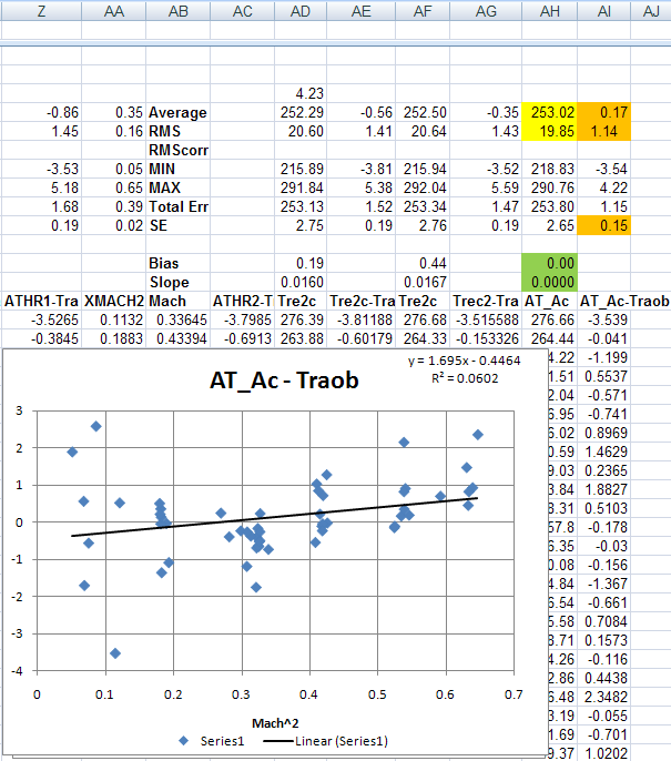
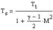
Figure 1a. Fifty-seven radiosonde comparisons WITHOUT a Mach Number correction.
Figure 1b. Fifty-seven radiosonde comparisons WITH a Mach Number correction. The green cells show the bias and slope of the Mach Number correction.
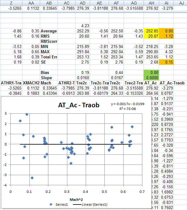
Figure 1c. Fifty-seven radiosonde comparisons a Mach Number correction correction applied in the analysis code to verify the correction. Note that the bias and slope of the Mach Number correction is zero (green cells).
Because we did radiosonde comparisons every 2 km from 2 km on up whenever the GV made a descent and ascent, we ended up with 104 potential comparisons within a range of 160 km of the aircraft. After these were editted for the criteria discussed above, including non-redundancy, the total number of comparisons was reduced 57. Figure 1a shows these 57 comparisons without a Mach Number correction, Figure 1b shows the same comparisons with a bias correction of 0.51 K and a slope correction of -0.0079, and Figure 1c just verifies that when the corrections were applied in the data analysis software that the bias and slope corrections go to zero. Note the 'slope correction' is really pressure altitude correction, but it is more closely tied to Mach Number Squared than it is to pressure altitude.
With the corrected avionics temperature (AT_Ac) in hand, we could calculate the MTP instrument gains for each observing frequency as:
G = [Counts (Horizon) - Counts (Target)] / [AT_Ac - Ttarget] in Counts/Kelvin.
where Counts (Horizon) and Counts (Target) are just the output of MTP when looking at the horizon (i.e., an in situ measurement in front of the GV) and the reference target. (The gain calculation is actually not this simple, but we'll spare you the details!) With the gains in hand, we could now do retrievals. After the first pass through all the flights, we calculate what we call a Window Correction Table (WCT). These are small temperature corrections that are applied to the measured brightness temperatures to correct for scan mirror side lobes. By design the WCT is always 0.0 K when the scan mirror elevation angle is zero, so this does not affect the flight level temperature calibration. Another retrieval pass is now made through all the flights with the WCT applied.
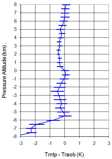
Figure 2a. Assessement of MTP performance relative to radiosondes BEFORE RAF correction.
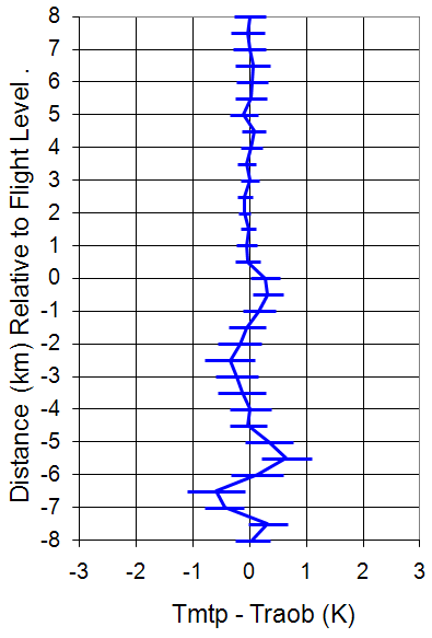
Figure 2b. Assessement of MTP performance relative to radiosondes AFTER RAF correction.
At this point we assess the accuracy of the MTP retrievals at all retrieval altitudes, not just flight level. This is done in Figure 2. In Figure 2a we show the MTP accuracy with respect to flight level for the 57 radiosonde comparisons. It is obvious that the retrieved MTP temperatures below the aircraft have a cold bias relative to radiosondes. This happens on the HIPPO flights because when the GV descends toward the ocean, the MTP 'sees' emission from the ocean which is colder that the air just above it. We have algorithms that can deal with this issue, but instead we took a simpler approach (to save time), which we call the RAF-correction. This has absolutely nothing to do with an NCAR research facility, but rather stands for REF-file After Fix (RAF). Since the accuracy assessment is telling us that the MTP retrieved temperatures are too cold below the aircraft, we simply do a sixth-order polynomial fit to determine the correction that gives the smallest over all bias with respect to radiosondes. This is shown in Figure 2b Note that this does create a small bias at flight level; however, our goal is to provide the best retrieved temperatures at all retrieval levels, not just flight level.
.JPG")


