A Summary of MTP Results for HIPPO-5
MJ Mahoney/JPL and Julie Haggerty/NCAR
Last Revision: March 26, 2012
We summarize on this web page, the results of the analysis of the Microwave Temperature Profiler (MTP) data obtained on the NSF/NCAR GV (NGV) during the HIPPO-5 field campaign. Its purpose is two-fold: to present the final MTP data with comments on each flight, and to discuss the excellent temperature calibration that was achieved.
Introduction
In our archived 'MP-files' we provide in the header record a comment urging users of these files to come to this web page for specific comments on the quality of the MTP data for each of the HIPPO-5 research flights. For this reason, we put the comments first in this summary. Following these comments, we provide information on how the temperature was calibrated (very successfully) for the HIPPO-5 campaign.
Comments on the HIPPO-5 MTP Final Data
The following table provides a link to a color-coded temperature curtain (CTC) for each of the HIPPO-5 research flights. More importantly, the table also provides a comments field where specific comments will be provided for each of the flights. Clicking on each thumbnail image will show the full-sized CTC image in a popup window, so that the image can be viewed while reading the comments. These comments are important because the rapid ascents and descents of the GV during the HIPPO campaigns degrade the quality of the MTP retrievals. On the other hand, this profiling -- as will be discussed below -- allowed very accurate temperature calibration.
First we provide an elaboration on the impact of rapid ascents and descents on the quality of the MTP retrievals. When retrievals are performed, the retrieval coefficients that we use assume that the pressure altitude is approximately constant. Clearly over an ~20 second MTP scan, this is not the case if the GV is profiling. Given a typical ascent or descent rate of ~150 m/s, 3 km are traversed in the vertical. (The actual distance is more like 2 km because not all of the 20 seconds is needed for measurements, but this is still unacceptably large.) We have tried to save as much of the ascent and descent data as possible by changing the editing threshold when it appears that the retrievals are consistent with the short level flight segments. This can be done by examining the behavior of the tropopause or the temperature field retrievals during ascent or descent compared to those during the level flight segments.
On each of the following CTC plots the x-axis is the Universal Time (UT) in kilo-seconds (ks), the left y-axis is the pressure altitude in kilometers (km), and the right y-axis is the pressure altitude in thousands of feet (kft). On the right is the color-coded temperature scale, which ranges from 170- 320 K. Also shown on each plot is the GV's altitude (black trace), the tropopause altitude (white trace), and a quality metric (gray trace at the bottom). The quality metric, which we call the MRI, ranges from 0 to 2 on the left pressure altitude scale. If the MRI is <1, we consider the retrieval to be reliable; if it is >1 the retrieval is less reliable, and users should contact us as to whether it can be used or not. The MTP final data have been edited to include retrievals with the MRI<0.8. If this excludes a specific time period that someone is interested in, they should contact us to see whether we can salvage that time period.
For most of the flights the CTC plots (which in fact are plotted using the archived data) are restricted to ±8 km from flight level. On a few flights this was increased so that higher tropopauses could be plotted; this was the case for several tropical flights.
| CTC | Comments |
|
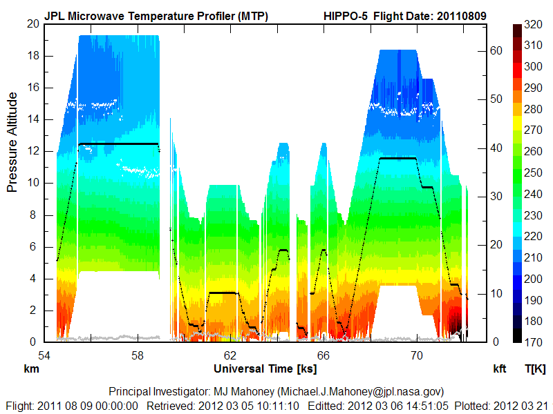
RF01 - 20110809 |
RMMA local flight The data for this flight looks excellent. There is a double tropopause early in the flight. |
|
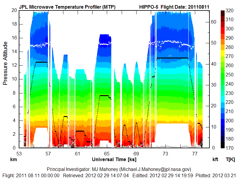
RF02 - 20110811 |
RMMA local flight The data for this flight looks excellent |
|
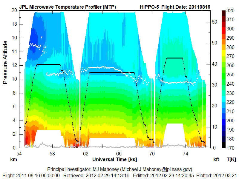
RF03 - 20110816 |
RMMA to Anchorage, Alaska The data for this flight looks excellent. |
|
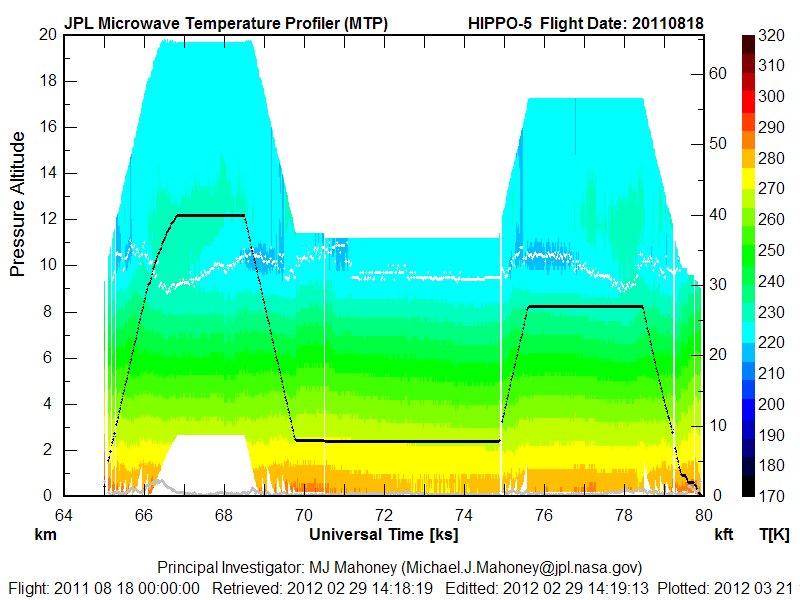
RF04 - 20110818 |
Anchorage, Alaska, to N Pole (aborted because of QCLS failure) This flight looks very good. On this aborted flight, the tropopause height variations look real as there is an obvious symmetry in the height variations. |
|
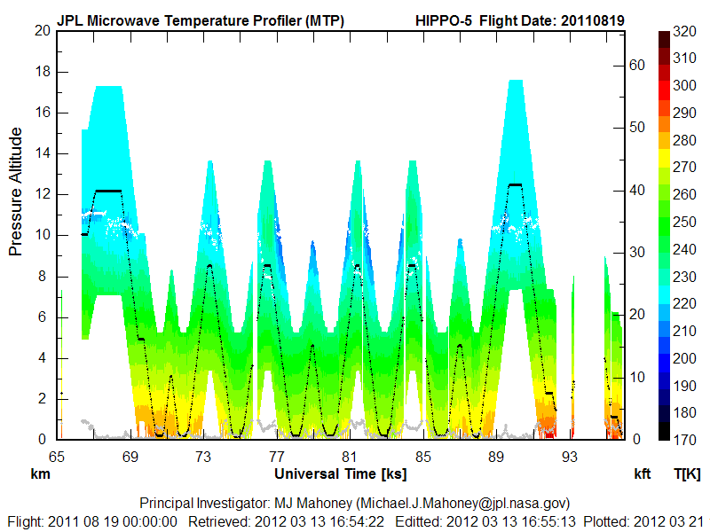
RF05 - 20110819 |
Anchorage, Alaska, to N Pole and back The data for this flight looks good. There is some 'ratiness' in the tropopause height caused by the rapid ascents and descents. Also, note that the temperatures at 8-10 km appear colder when the GV is low compared to when it is high. This is caused by the rapid ascents and descents. The best estimate of the tropopause height and temperature is obtained when the GV is high. |
|
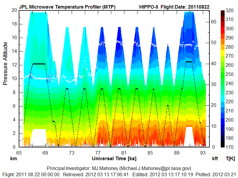
RF06 - 20110822 |
Anchorage, Alaska, to Kona, Hawaii The data for this flight look excellent. |
|
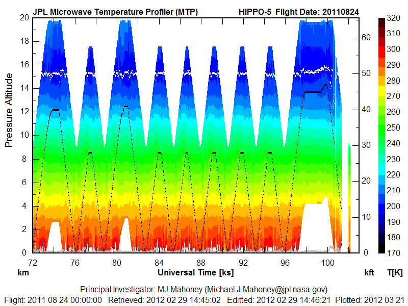
RF07 - 20110824 |
Kona, Hawaii, to Roratonga, Cook Islands The data for this flight looks excellent. The retrieval range was increased to ±10 km from flight level in order to show the tropopause. |
|
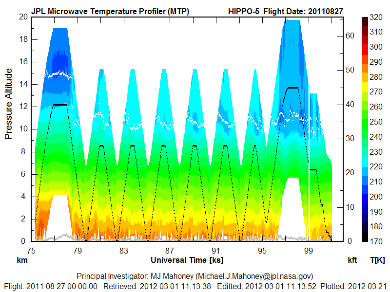
RF08 - 20110827 |
Roratonga, Cook Islands to Christchurch, New Zealand The retrievals for this flight look excellent. |
|
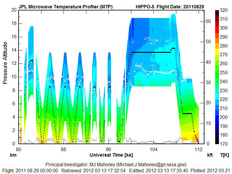
RF09 - 20110829 |
Christchurch, NZ to S Pole and back The retrievals are good. However, this data suffers from the same ascent and descent issues discussed for the N Pole flight on 20010819 (RF05). The retrievals should not be trusted from 95-101 ks because the measured brightness temperatures appeared to contain interference. |
|
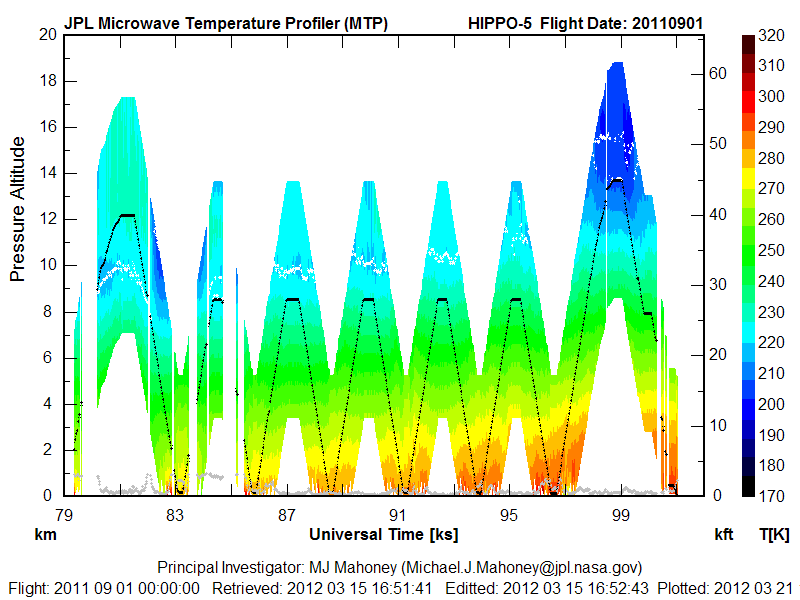
RF10 - 20110901 |
Christchurch, NZ to Rarotonga, Cook Islands The data for this flight are fine. |
|
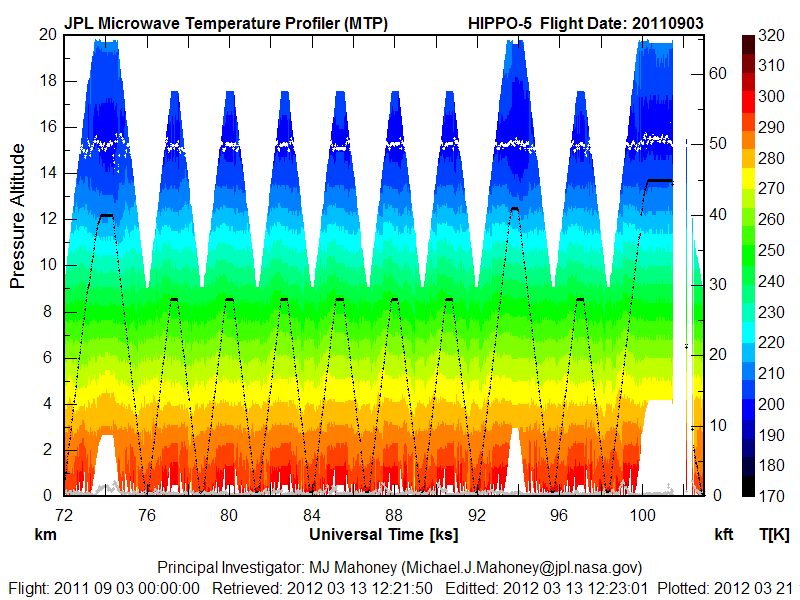
RF11 - 20110903 |
Rarotonga, Cook Islands to Kona, Hawaii The data for this flight are excellent; it is a 'poster' flight. Retrievals are shown +/-10 km from flight level to show the tropopause. |
|
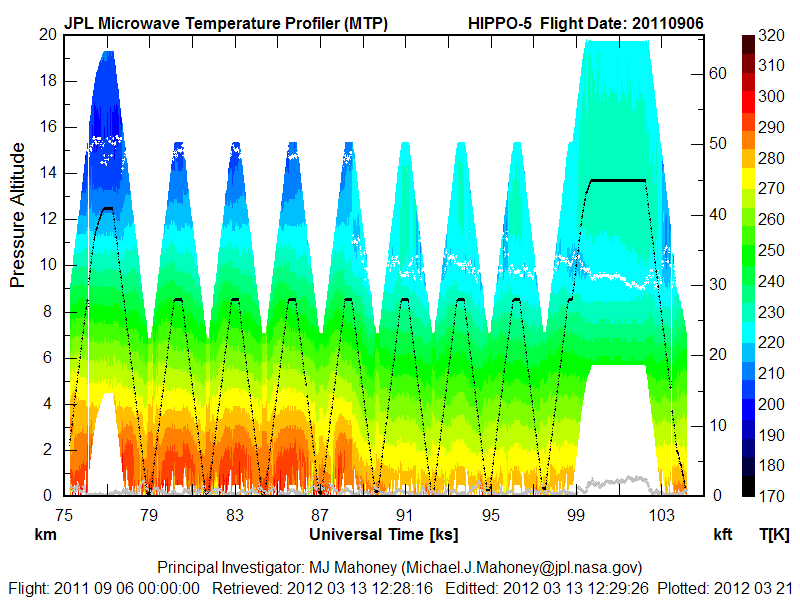
RF12 - 20110906 |
Kona, Hawaii, to Anchorage, Alaska The data for this flight are excellent. |
|
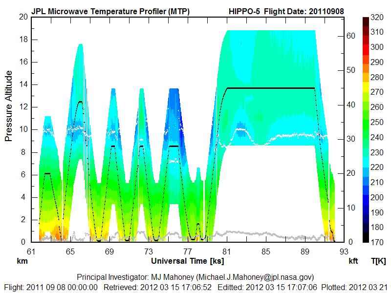
RF13 - 20110908 |
Anchorage, Alaska, to N Pole and back Like the other polar flights, this flight has compromised retrievals due to the rapid ascents and descents. In addition the brightness temperatures showed interference from 71-86 ks, so these retrievals should not be trusted. |
|
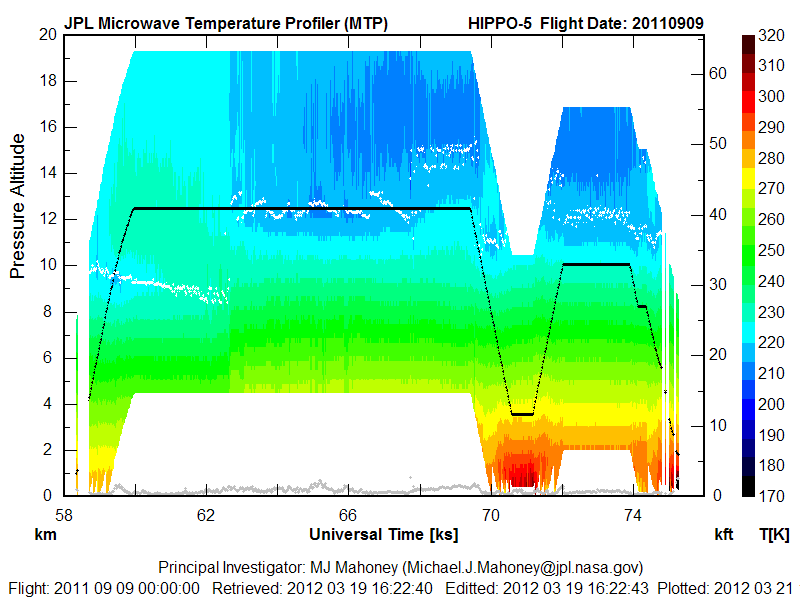
RF14 - 20110909 |
Transit flight from Anchorage, Alaska to RMMA This flight is of good quality. |
HIPPO-5 Temperature Calibration
1) Some Background
For more than two decades the MTP team has been refining techniques for calibrating in situ temperature measurements made aboard research aircraft by performing comparisons with radiosondes launched near the aircraft's flight track. Initially this was done by hand, and could involve as much as a day for a single comparison because of the tedious quality control procedures that had to be implemented (such as limiting pressure altitude excursions during the comparisons, restricting allowable pitch and roll changes, and checking for radiosonde temporal and spatial variability). About a decade ago these procedures were largely automated, but the comparisons were made for the entire MTP-retrieved temperature profile at that time, not just at flight level.
Even though the MTP did not participate in the T-Rex campaign, we were asked if the MTP temperature calibration techniques could be applied to the the research and avionics temperatures measured during T-Rex so that differences in these temperatures could be resolved. During T-Rex the GV flew from RMMA to near Independence, CA, where it spent most of its flight time. In addition to the NWS soundings on transit, Leeds University frequently launched radiosondes from Independence, CA (INCA), so we had a wealth of soundings with which to do comparisons. All of the radiosondes used had an accuracy of ±0.3 K. As described on another web page, we found that both the research temperature Tres (ATRL) and the avionics temperature Tavi (AT_A) had substantial warm biases with respect to radiosondes launched near the GV flight track (Tavi - Traob = 1.21 ± 0.12, and Tres - Traob = 2.37 ± 0.12, respectively). While Tres has the largest warm bias, we also found that the Tavi warm bias is very significantly pressure altitude dependent.
This work to understand the T-Rex in situ temperatures opened the door to a new approach for doing the MTP temperature calibration. As mentioned above we had previously compared the entire retrieved temperature profile to radiosondes, not just the flight level temperature. This often required several retrieval iterations through all the flights to achieve acceptable results. After doing the T-Rex comparisons, it was realized that, if the flight level temperature was calibrated independently of the MTP data, less work would be needed. (This is the case because previously we applied a correction to the in situ temperature measurement called OATnavCOR. Therefore, every time that OATnavCOR changed we would have to recalculate the instrument gain. If the flight level temperature is accurately calibrated from the start, then OATnavCOR is always 0.0 K, and the instrument gains do not have to be recalculated. This saves a lot of effort.)
We have continued to refine the temperature calibration techniques that we developed for T-Rex on subsequent GV campaigns. There are other web pages that describe this procedure for START-08, HIPPO-1, HIPPO-2, HIPPO-3, PREDICT, DC3-Test and HIPPO-4.
Before discussing the calibration procedure for the HIPPO-5 field campaign, we will first provide a little background. During the HIPPO field campaigns the GV was for the most part continuously profiling the troposphere (and sometimes the lower stratosphere). This was a significant concern for a number of reasons:
- First, in order to obtain good temperature profile retrievals, the MTP requires that the pressure altitude of the aircraft be relatively constant during the course of a ~20 second scan. This was blatantly not the case when the GV is behaving like an over-sized atmospheric yoyo.
- Second, related to this is the fact that we have typically averaged 3 -7 scans to beat down noise introduced by mesoscale temperature variations. Such averaging would be impossible during rapid descents and ascents.
- Third, in the past we have flatly refused to do radiosonde comparisons in the troposphere because of the high lapse rate, and therefore sensitivity to altitude excursions.
- Fourth, in order to do radiosondes comparisons, you need radiosondes. Since most of the HIPPO flights were in radiosonde sparse regions (the Arctic, Antarctic and Pacific Ocean), obtaining enough comparisons to achieve good statistics could be difficult.
- Fifth, careful consideration needs to be given to the dependence of the temperature recovery factor on Mach Number. There is no way that a constant temperature recovery factor can be used when an aircraft (and its in situ temperature probes) are profiling the atmosphere.
For these reasons our hand was forced. Normally when we do radiosonde comparisons, we do them at the time of great-circle closest approach to the radiosonde launch site. We are also careful to make sure that no one radiosonde comparison overly weights the statistics. For example, suppose that the GV was taking off or landing at an airfield where radiosondes were launched. The "closest approach" algorithm might produce multiple times of closest approach during frequent turns. We would edit out these additional comparisons to avoid overly weighting the statistics to this site. Given the sparsity of oceanic and polar radiosondes, and the desire to have good statistics, we decided to try a new approach for the HIPPO campaigns (and other campaigns where atmospheric profiling is common). Instead of using the great-circle time of closest approach to make the comparison, we decided to do comparisons every 1 km in altitude from 2 km on up with the closest radiosonde launch site that was available. (If the closest radiosonde launch site was very distant, we had a filter that would exclude soundings beyond a specified distance threshold.) This approach would increase the number of potential comparisons by nearly an order of magnitude. But equally as important, it would allow us to assess whether any of the in situ temperature measurements had a pressure altitude dependence, which, as we remarked above, was the case for the avionics temperature during T-Rex. In addition to allowing tropospheric radiosonde comparisons, we would also be forced to abandon averaging of scans to beat down the mesoscale temperature noise, since (when profiling) the temperature change due to altitude change completely dominates any change due to mesoscale temperature variations.
2) What We Did For HIPPO-5
Based on our experience from the HIPPO-2, HIPPO-3 and HIPPO-4 temperature calibration, where the avionics temperature produced the best results, we decided to proceed with the temperature calibration for HIPPO-5 using the avionics temperature. This would save time waiting for the research temperatures to be calibrated (sic). We also used procedures to calibrate the in situ temperature as a function of Mach Number squared, instead of a simple pressure altitude dependence. Using this procedure we found that the avionics temperature (AT_A), when forced to agree with 89 radiosonde comparisons near the GV flight track had the following corrected (AT_Ac) value:
AT_Ac = AT_A -2.19970 * Mach2 +0.9019
The Mach Number corrections for these corrected temperature measurements are important; it varies from -0.79 K to +0.64 K depending on the Mach Number.
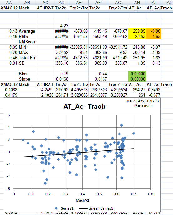
Figure 1a. One hundred and forty-seven radiosonde comparisons WITHOUT a Mach Number correction.
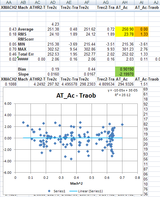
Figure 1b. One hundred and thirty-eight radiosonde comparisons WITH a Mach Number correction. The green cells show the bias and slope of the Mach Number correction.
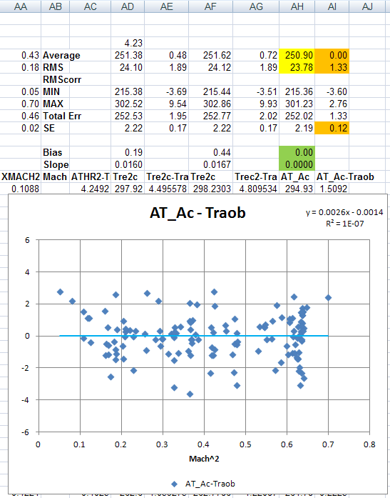
Figure 1c. One hundred and thirty-eight radiosonde comparisons with a Mach Number correction applied in the analysis code to verify the correction. Note that the bias and slope of the Mach Number correction is zero (green cells).
Because we did radiosonde comparisons every 1 km from 2 km on up whenever the GV made a descent and ascent, we ended up with 147 potential comparisons within a range of 320 km of the aircraft. After these were edited for the criteria discussed above, including non-redundancy, the total number of comparisons was reduced 138. Figure 1a shows these 147 comparisons without a Mach Number correction, Figure 1b shows the edited 138 comparisons with a bias correction of 0.9019 K and a slope correction of -2.1997, and Figure 1c just verifies that when the corrections were applied in the data analysis software that the bias and slope corrections go to zero. Note the 'slope correction' is really pressure altitude correction, but it is more closely tied to Mach Number Squared than it is to pressure altitude.
With the corrected avionics temperature (AT_Ac) in hand, we could calculate the MTP instrument gains for each observing frequency as:
G = [Counts (Horizon) - Counts (Target)] / [AT_Ac - Ttarget] in Counts/Kelvin.
where Counts (Horizon) and Counts (Target) are just the output of the MTP when looking at the horizon (i.e., an in situ measurement in front of the GV) and the reference target. (The gain calculation is actually not this simple, but we'll spare you the details!) With the gains in hand, we could now do retrievals. After the first pass through all the flights, we calculate what we call a Window Correction Table (WCT). These are small temperature corrections that are applied to the measured brightness temperatures to correct for scan mirror side lobes. By design the WCT is always 0.0 K when the scan mirror elevation angle is zero, so this does not affect the flight level temperature calibration. Another retrieval pass is now made through all the flights with the WCT applied.
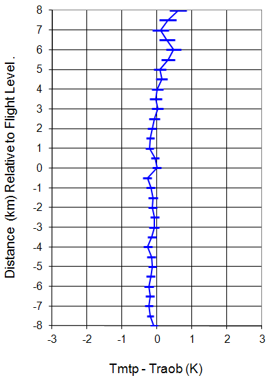
Figure 2a. Assessement of MTP performance relative to radiosondes BEFORE RAF correction.
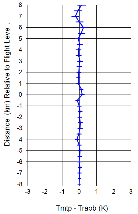
Figure 2b. Assessement of MTP performance relative to radiosondes AFTER RAF correction.
At this point we assess the accuracy of the MTP retrievals at all retrieval altitudes, not just flight level. This is done in Figure 2. In Figure 2a we show the MTP accuracy with respect to flight level for the 173 radiosonde comparisons. (This is less than the original 198 comparisons because we wanted to exclude comparisons on the two flights where there was obvious interference (20110829 and 20110908).) It is obvious that there is a small warm bias more than 5 km above flight level. The reason for this is that when the GV is flying at low altitudes the MTP is not able to accurately resolve sharp tropopause features; it will over-estimate the temperature (see Figure 4a below). There is also a slight cold bias below the aircraft. We believe that this is due to the ocean temperature being colder than the air temperature just above it. We have an algorithms that can deal with this issue, but instead we took a simpler approach (to save time), which we call the RAF-correction ( REF-file After Fix, or RAF). Since the accuracy assessment is telling us that the MTP retrieved temperatures are too cold below the aircraft and too warm above the aircraft, we simply do a sixth-order polynomial fit to determine the correction that gives the smallest over-all bias with respect to radiosondes. This is shown in Figure 2b Note that this does create a very small bias at flight level; however, our goal is to provide the best retrieved temperatures at all retrieval levels, not just flight level.
This said, we decided not to apply the RAF correction! Why? Because over-estimating the temperature near the tropopause is primarily a problem when flying low in the tropics. Applying the RAF correction to all flights, including those outside the tropics, would then cause temperatures outside the tropics to be under-estimated. And in fact, had the RAF correction been determined using only tropical flights, the correction would likely to have been much larger. We decided not to calculate a tropics-only RAF correction since the performance without a RAF correction is already excellent (<0.5 K ±8 km from flight level).
3) A Sanity Check
When we calibrate the in situ temperature, there are a number of sanity checks that we perform. In part these have to do with deciding which, if any, of the possible RAOB comparisons should be excluded. The only ground rule on these checks is that they be completely objective. Two obvious checks involve looking at how the bias and rms of the nav temperature minus the RAOB temperature (Tnav - Troab) vary as a function of a temperature threshold or as a function of the range or distance from the RAOB launch site.
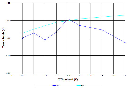
Figure 3a. A temperature threshold comparison.
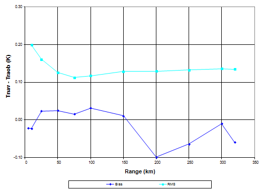
Figure 3b. A range threshold comparison.
Figure 3a shows a temperature threshold comparison.Basically, the Tnav - Traob values for each comparison are checked against a threshold temperature. For example, if the threshold temperature is 3 K then all differences whose absolute value exceeds 3 K are removed and the bias and rms of the remaining comparisons are calculated. Figure 3a shows the results. Often when this is done as the threshold gets smaller and smaller the rms will tend to go up because of the decreasing statistics. For HIPPO-5 however because we had so many accurate comparisons, the rms continued to monotonically decrease, and in fact from this plot we can safely say that there is no statistically significant bias, since the light cyan curve representing the rms lies above the blue curve representing the bias.
Figure 3b shows a range threshold comparison. In this case comparisons exceeding a specified distance from the RAOB launch site are removed and the bias and rms of the remaining comparisons is calculated. During HIPPO-5 there were few comparisons at close range, which is to be expected when flying over mainly oceanic regions. So in this comparison, the rms begins to increase at distances closer than 75 km. Again, we can say that there is no statistically significant bias in Tnav - Trms because the absolute value of the bias is always <0.1 K while the rms is always >0.1 K.
Another objective comparison technique is to exclude comparisons within some specified distance from the tropopause to avoid obvious temperature changes. In fact when we perform the RAOB and nav temperature comparison, we generate an image showing the RAOB launched before and after the GV flew by the RAOB launch site (see yellow and blue traces in Figure 4, as well as a temporally interpolated profile to the time of the fly by (white profile). We then superimpose of these RAOB profiles the MTP measured temperature profile (cyan) to assess whether there is any temporal temperature variability.
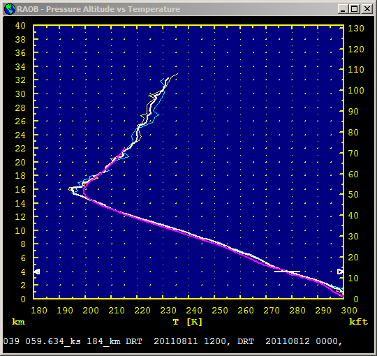
Figure 4a. Comparisons of MTP temperature profile (magenta) to temporally interpolated profile (white) from Del Rio, Texas (DRT).
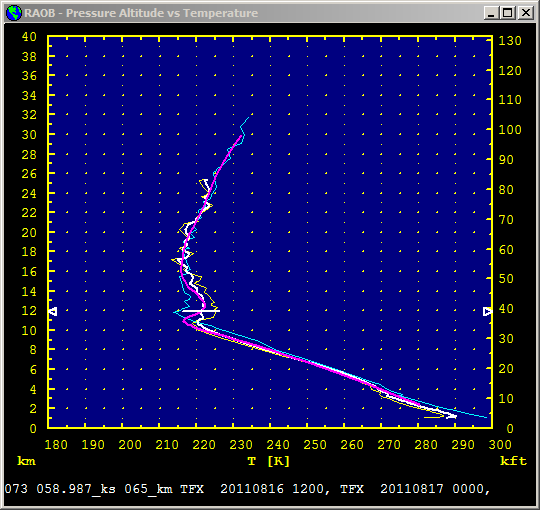
Figure 4b. Comparisons of MTP temperature profile (magenta) to temporally interpolated profile (white) from Grand Falls, Montana (TFX).
In Figure 4a it is clear that there is little temperature variability between the before (yellow) and after (cyan) RAOBs up to about 22 km. Notice how, because the GV is flying at 4 km, the MTP is not able to resolve the tropopause 12 km higher. It therefore over-estimates the temperature at that altitude, and this is what we were referring to in our discussion of the RAF correction above.
In Figure 4b we see a situation in which there is an obvious temperature change in the before (yellow) and after (cyan) soundings above ~10 km. Since the GV was flying at 12 km, it would be reasonable to exclude this comparison. However, notice that the temporally interpolated sounding (white) for the time of the comparison is in excellent agreement with the in situ aircraft measurement (center of horizontal white bar at 12 km). So you might want to keep the comparison, but that wouldn't be objective. There is certainly no guarantee that the temporal variability is linear.


