A Summary of MTP Results for DC3-Test
MJ Mahoney/JPL and Julie Haggerty/NCAR
Last Revision: October 04, 2011
We summarize on this web page, the results of the analysis of the Microwave Temperature Profiler (MTP) data obtained on the NSF/NCAR GV (NGV) during the DC3-Test field campaign. Its purpose is two-fold: to present the final MTP data with comments on each flight, and to discuss the excellent temperature calibration that was achieved.
Introduction
In our archived 'MP-files' we provide in the header record a comment urging users of these files to come to this web page for specfic comments on the quality of the MTP data for each of the DC3-Test research flights. For this reason we put the comments first in this summary. Following these comments, we provide information on how the temperature was calibrated (very successfully) for the DC3-Test campaign.
Comments on the DC3-Test MTP Final Data
The following table provides a link to a color-coded temperature curtain (CTC) for each of the DC3-Test flights. More importantly, the table also provides a comments field where specific comments will be provided for each of the flights. Clicking on each thumbnail image will show the full-sized CTC image in a popup window, so that the image can be viewed while reading the comments. These comments are important because -- as will be discussed below -- the MTP retrieval coefficients did not capture strong ground inversions (although the MTP could 'see' them), and because when the GV was flying low, the MTP beam would 'see' excess emission from the ground.
First we provide an elaboration on the impact of rapid ascents and descents on the quality of the MTP retrievals. This has had a big impact on the HIPPO field campaigns when the GV is continuously profiling, but this was less the case during DC3-Test. When retrievals are performed, the retrieval coefficients that we use assume that the pressure altitude is approximately constant. Clearly over an ~20 second MTP scan, this is not the case. Given a typical ascent or descent rate of ~1500 ft/min (25 ft/sec, 8 m/s), 160 meters are traversed in the vertical. (The actual distance is more like ~200 meters because not all of the 20 seconds is needed for measurements, but this is still unacceptably large.) We have tried to save as much of the ascent and descent data as possible by changing the editting threshold when it appears that the retrievals are consistent with the short level flight segments. This can be done by examining the behaviour of the tropopause or the temperature field retrievals during ascent or descent compared to those during the level flight segements.
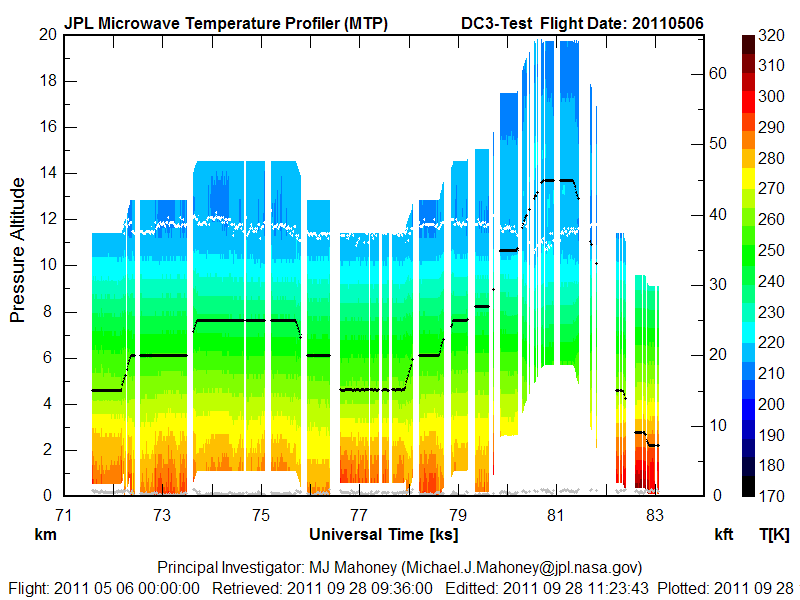
On each of the following CTC plots the x-axis is the Universal Time (UT) in kilo-seconds (ks), the left y-axis is the pressure altitude in kilometers (km), and the right y-axis is the pressure altitude in thousands of feet (kft). On the right is the color-coded temperature scale, which ranges from 170- 320 K. Also shown on each plot is the GV's altitude (black trace), the tropopause altitude (white trace), and a quality metric (gray trace at the bottom). The quality metric, which we call the MRI, ranges from 0 to 2 on the left pressure altitude scale. If the MRI is <1, we consider the retrieval to be reliable; if it is >1 the retrieval is less reliable, and users should contact us as to whether is can be used or not.
For most of the flights the CTC plots (which in fact are plotted using the archived data) are restricted to ±8 km from flight level. On a few flights this was increased so that higher tropopauses could be plotted.
| CTC | Comments |
| TF01 - 20110502 | Local test flight from RMMA This short flight provided no useful MTP data |
| TF02 - 20110504 | Local test flight from RMMA This flight provided no useful MTP data. Examination of the engineering data showed that the +8 V voltage regulator was not functioning properly. It was repaired and all the remaining flights obtained good data. |
|
TF03 - 20110506 |
Local test flight from RMMA The retrievals were excellent except after ~81.5 ks on the GV's final descent. The MRI threshold was set to 0.3 in the archived data to avoid showing scans with excessive thermal emission from the ground. |
|
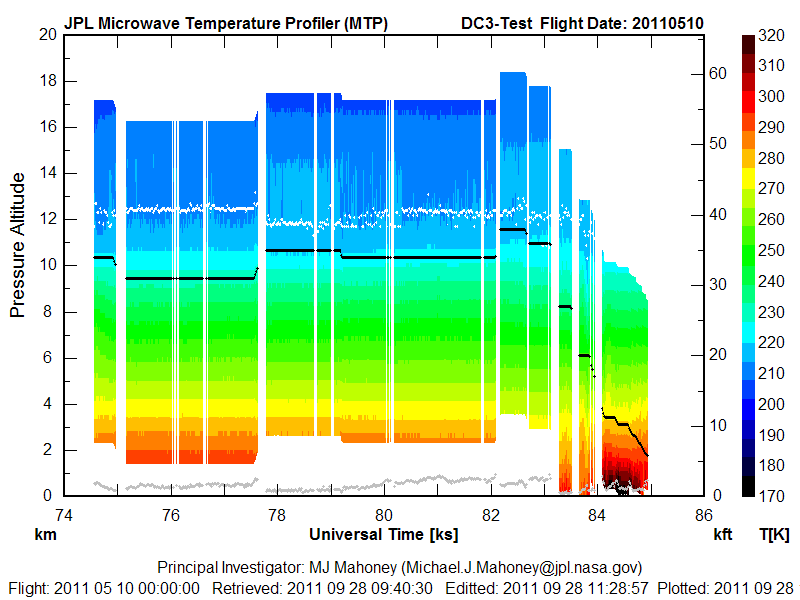
TF04 - 20110510 |
Local test flight from RMMA The retrievals were excellent except after ~83.5 ks on the GV's final descent. The MRI was not used to edit any data with excess thermal emission from the ground. So data beyond 83.5 ks should only be used above the aircraft. We have the ability to modify the retrievals to handle these conditions, but it requires a lot of extra effort which we felt wasn't justified for test flights. |
|
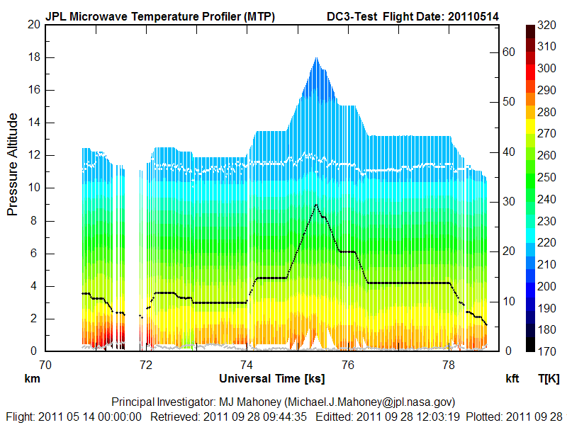
TF05 - 20110514 |
Local test flight from RMMA The retrievals are excellent above the GV for this flight. A ground inversion appears below ~4 km, which affects the downward retrieval. Because the 0 hr and 12 hr radiosondes did not capture the inversion, they did not do a good job of retrieving it. In such a situation we would synthesize an inversion on the radiosondes before calculating retrieval coefficients. We did not take this extra effort because it was not justified for test flights. |
|
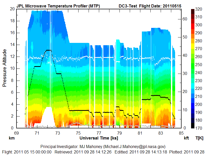
TF06 - 20110515 |
Local test flight from RMMA The retrievals are excellent above the GV for this flight, although more work could improve the retrievals near 72 ks.. A strong ground inversion appears below ~3 km, which affects the downward retrievals from 74-81 ks. Because the 0 hr and 12 hr radiosondes did not capture this inversion, they did not do a good job of retrieving it, and this was exacerbated by the ground emission. We did not take the effort to synthesize an inversion on the radiosondes before calculating retrieval coefficients, because we felt that it was not justified for test flights. |
DC3-Test Temperature Calibration
1) Some Background
For nearly two decades the MTP team has been refining techniques for calibrating in situ temperature measurements made aboard research aircraft using radiosondes launched near the aircraft's flight track. Initially this was done by hand, and could involve as much as a day for a single comparison because of the tedious quality control procedures that had to be implemented (such as limiting pressure altitude excursions during the comparisons, restricting allowable pitch and roll changes, and checking for radiosonde temporal and spatial variability). About a decade ago these procedures were largely automated, but the comparisons were made for the entire MTP-retrieved temperature profile at that time, not just at flight level.
Even though the MTP did not participate in the T-Rex campaign, we were asked if the MTP temperature calibration techniques could be applied to the the research and avionics temperatures measured during T-Rex so that differences in these temperatures could be resolved. During T-Rex the GV flew from RMMA to near Independence, CA, where it spent most of its flight time. In addition to the NWS soundings on transit, Leeds University frequently launched radiosondes from Independence, CA (INCA), so we had a wealth of soundings with which to do comparisons. All of the radiosondes used had an accuracy of ±0.3 K. The results are described on another web page.
This work to understand the T-Rex in situ temperatures opened the door to a new approach for doing the MTP temperature calibration. As mentioned above we had previously compared the entire retrieved temperature profile to radiosondes, not just the flight level temperature. This often required several retrieval iterations through all the flights to achieve acceptable results. It was realized that if the flight level temperature was calibrated independently of the MTP data that less work would be needed.
We have continued to refine the temperature calibration techniques that we developed for T-Rex on subsequent GV campaigns, and we believe that our results represent the most accurate in situ temperature calibration available on any airborne platform. There are other web pages that describe this procedure for START-08, HIPPO-1, HIPPO-2, HIPPO-3, and PREDICT.
2) What We Did For DC3-Test
For DC3-Test there were five in situ temperature measurements that were available for radiosondes comparisons: AT_A, ATHL1, ATHL2, ATHR1, and ATHR2, but because final data was not yet available, we decided to do this analysis using AT_A -- the avionics temperature-- because it would not change in the final archive. (AT_A was also the most accurate temperature based on prior analysis.) Since the correction from total temperature (Tt) to static temperature (Ts) involves Mach Number squared (see this webpage for more information; this equation ignores the recovery factor):
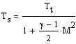
we forced AT_A to agree with radiosondes measurements by calculating a corrected AT_Ac temperature given by:
AT_Ac = AT_A * (1 - 0.00922 * M2) + 0.885
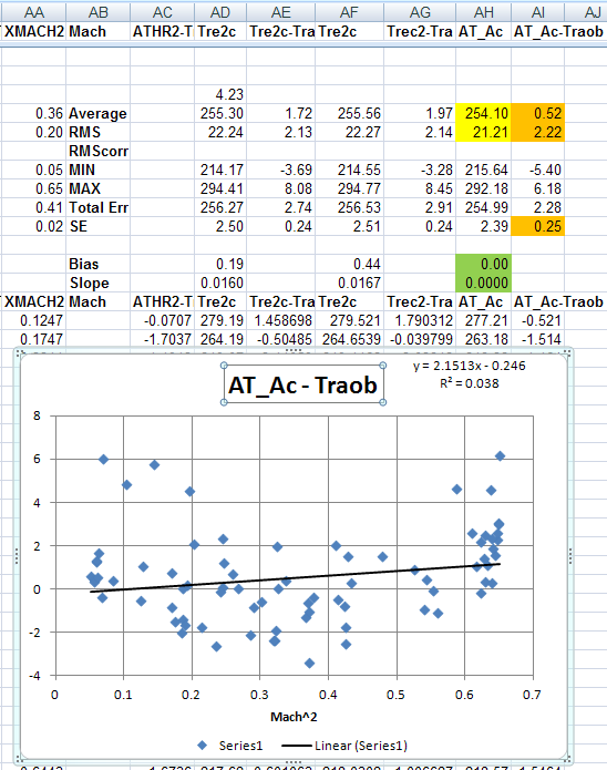
Figure 1a. Fifty-seven radiosonde comparisons WITHOUT a Mach Number correction.
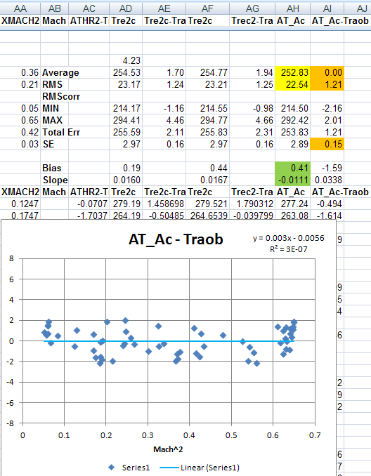
Figure 1b. Fifty-seven radiosonde comparisons WITH a Mach Number correction. The green cells show the bias and slope of the Mach Number correction.
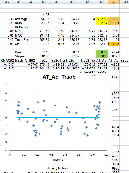
Figure 1c. Fifty-seven radiosonde comparisons a Mach Number correction correction applied in the analysis code to verify the correction. Note that the bias and slope of the Mach Number correction is zero (green cells).
Because we did radiosonde comparisons every 1 km from 1 km on up whenever the GV made a descent and ascent, we ended up with 80 potential comparisons within a range of 320 km of the aircraft; Figure 1a shows these 80 comparisons without a Mach Number correction and no editting. After these were editted for the criteria discussed above, including non-redundancy, the total number of comparisons was reduced to 62; Figure 1b shows the comparisons with a bias correction of 0.41 K and a slope correction of -0.0101, and Figure 1c just verifies that when the corrections were applied in the data analysis software that the bias and slope corrections go to zero. Note the 'slope correction' is really pressure altitude correction, but it is more closely tied to Mach Number Squared than it is to pressure altitude.
With the corrected avionics temperature (AT_Ac) in hand, we could calculate the MTP instrument gains for each observing frequency as:
G = [Counts (Horizon) - Counts (Target)] / [AT_Ac - Ttarget] in Counts/Kelvin.
where Counts (Horizon) and Counts (Target) are just the output of MTP when looking at the horizon (i.e., an in situ measurement in front of the GV) and the reference target. (The gain calculation is actually not this simple, but we'll spare you the details!) With the gains in hand, we could now do retrievals. After the first pass through all the flights, we calculate what we call a Window Correction Table (WCT). These are small temperature corrections that are applied to the measured brightness temperatures to correct for scan mirror side lobes. By design the WCT is always 0.0 K when the scan mirror elevation angle is zero, so this does not affect the flight level temperature calibration. Another retrieval pass is now made through all the flights with the WCT applied.
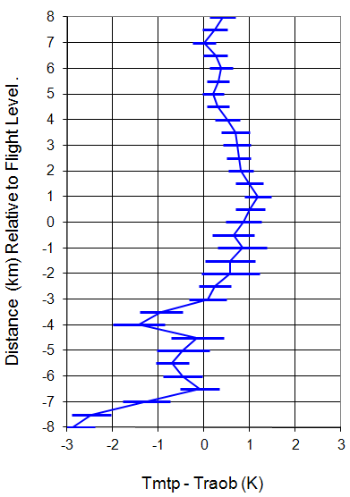
Figure 2a. Assessement of MTP performance relative to radiosondes BEFORE RAF correction.
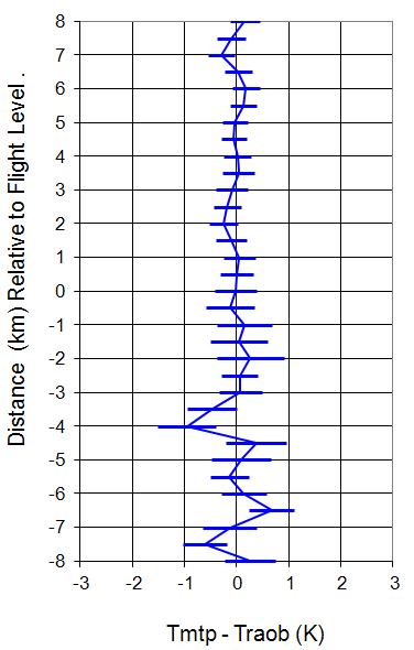
Figure 2b. Assessement of MTP performance relative to radiosondes AFTER RAF correction.
At this point we assess the accuracy of the MTP retrievals at all retrieval altitudes, not just flight level. This is done in Figure 2. In Figure 2a we show the MTP accuracy with respect to flight level for the 62 radiosonde comparisons. It is obvious that the retrieved MTP temperatures below the aircraft have a cold bias relative to radiosondes. This happens on the DC3-Test flights because when the GV descends toward the ground, there is a strong inversion on several flights which the MTP 'sees', but which the radiosondes (because of their launch times) do not 'see.' Similarily, because of degraded vertical resolution near the tropopause, the MTP tends to over-estimate the temperature there. We have algorithms that can deal with this issue, but instead we took a simpler approach (to save time), which we call the RAF-correction. This has absolutely nothing to do with an NCAR research facility, but rather stands for REF-file After Fix (RAF). Since the accuracy assessment is telling us that the MTP retrieved temperatures are too cold below the aircraft, we simply do a sixth-order polynomial fit to determine the correction that gives the smallest over all bias with respect to radiosondes. This is shown in Figure 2b Note that this does create a small bias at flight level; however, our goal is to provide the best retrieved temperatures at all retrieval levels, not just flight level. We decided not to apply the RAF correction because the bias below the aircraft is real; the MTP measurements are correct and the RAOBs are incorrect.


