Introduction
Of vital importance in the understanding of surface fluxes is the ability to relate the flux measured at some height above the ground with the specific area of the surface to which this flux corresponds. For micrometeorological flux measurements this relationship varies with atmospheric conditions.
The common micrometeorological techniques for determining surface fluxes yield flux magnitude and sense but give little information about the location of the area source or sink of the scalar. Knowledge of the upwind fetch is necessary to estimate the location of the actual surface which is involved in the emission or deposition of the scalar investigated. It is this proportionally-contributing area of surface which is described as the flux footprint. The footprint expand or contracts, elongates or widens with different conditions of stability and wind speed. The footprint is smaller when the measurements are made closer to the surface and larger when the measurement height is increased.
Micrometeorological rules-of-thumb probably suffice when the surface is uniform in its deposition/emission characteristics. Such rules generally specify minimum uniform surface fetches. Several models exist which can be used to predict the footprint. However, there is a need for readily applicable models which can be used to design experiments and interpret results for varying conditions. Such models require experimental data sets to validate them under a range of atmospheric conditions. The FOOTPRINT92 field program was undertaken to provide such an experimental data set.
The basic design of the ASTER-supported field study involved the controlled release of sulfur hexafluoride from a crosswind line source and the measurement of the vertical flux at different heights and distances downwind. Fast response SF6 sensors were used with sonic anemometers to measure the SF6 fluxes by eddy correlation. The ASTER facility also served to determine the micrometeorological environment.
Operations
Field Site
The terrain at the research site was moderately flat. To the northwest, the direction of the prevailing wind, there was approximately 8 kilometers before any significant change of altitude. The ground had a patchy covering of senescent grasses with bare sand exposed in approximately 15% of the area. The vegetation was dominated by sagebrush, one to two meters high, scattered approximately 5 meters apart, and occupying approximately 20% of the area. Figures 3, 4, 5 and 6 show the location and configuration of the ASTER array. The array was established between the 800 meter arc road and the 1600 meter arc road of the Hanford diffusion grid, aligned along an axis bearing 65 degrees west of true north, corresponding to the direction of the prevailing wind.
Stations were marked at 50m, 100m, 175m, 250m, 500m, and 750m from the 400 meter-long SF6 release line. This line was placed 1 meter above the ground at right angles to the prevailing wind direction. It was initially planned to make flux measurements first at the 50m, 100m, 175m and 250m stations during unstable conditions and then at the 50m, 250m, 500m, and 750m stations during stable conditions. Subsequently it was decided to forego the reconfiguration and to maintain the original configuration throughout the entire deployment. Four flux stations were established at 50m, 100m, 175m, and 250m. Each station had a 10m tower equipped with a 3-D sonic anemometer, a fast temperature sensor and a fast response SF6 detector. In addition, at the 50m station there was a wind profile tower and at the 250m station there was a psychrometer profile tower and the radiation and soil heat flux array.
After the array was established, the orientations of the booms of the prop-vanes and of the sonic anemometers were determined using a theodolite set to true north by means of solar sighting and an ephemeris. This defined the true bearing of the prop-vanes as the sensor encoders were accurately aligned with the boom. However for the sonic anemometers the transducer alignment did not accurately correspond to that of the boom. Hence for the sonic anemometers this bearing was used as a nominal value and was later corrected to the true value by comparing the sonic anemometer and the prop-vane data. (see the section on Alignment)
Special Deployment Aspects
The FOOTPRINT92 deployment offered several special problems. Because of the distributed nature of the deployment, the power distribution and data gathering system had to be modified. The four flux stations each had to be supplied with power and connected by fiber optical cable to the ASTER base. The power was generated at the ASTER base by two 15 KVA diesel generators supplied, fueled and maintained by the Hanford Facility. The generators were refueled daily and sequentially shut down for maintenance every third day for a brief period. Prior to the shut down periods the ASTER power load had to be adjusted, bringing down nonessential computer resources and air conditioning. During the setup phase of the deployment, until the appropriate procedure was established, misbehavior of the Uninteruptable Power Supply led to considerable difficulties. The fiber-optic cable connection from the four flux stations also gave problems until the optical intensity was increased and the discrimination level decreased.
Operational Period
The ASTER system was fully operational by June 2nd and for the duration of the field program data was continuously acquired from all the ASTER-maintained sensors. For the first portion of the field study, during operations 1 and 2 (ops1 and ops2), the flux systems were positioned at a height of 10 meters. During the second portion of the field study (ops3) the flux systems were positioned at a height of 5 meters. The field program was continued until July 1st, 1992.
Sensors
Table 1 lists the sensors deployed for FOOTPRINT92.
Sonic Anemometers
From the beginning of the deployment until June 22nd (jd174), the sonic anemometers operated at 10 m. From that day until the end of the deployment the sonic anemometers operated at 5 m.
The sonic anemometers required attention throughout the deployment. A radical problem to be noted involved the ATI devices. On June 15th (jd167), the ATI model K at the 50m station, "atiK.50.10," was found to be very noisy and the spare sensor, the older ATI model S, "atiS.50.10" was substituted. This ATI model S also had problems over the next several days. On June 19th (jd171), a transducer had to be replaced on the ATI model S and a vertical offset resulted. On June 21st (jd 173), the ATI model S was again replaced by the original ATI model K which had been returned to the manufacturer for repair. The ATI model K was then adjusted to obtain clean signals and a proper zero calibration. This sonic anemometer operated, with occasional problems, for the remainder of the project.
Fast Thermometers
From the beginning of the deployment until June 22nd (jd174), the fast thermometers operated at 10 m. From that day until the end of the deployment the fast thermometers operated at 5 m.
The fast thermometers performed well throughout the deployment
Krypton Hygrometers
Campbell Scientific krypton hygrometers were operated with the flux arrays at the 50m and the 250m flux stations. They were calibrated prior to the deployment and performed well throughout the program.
Prop-Vanes
The prop-vanes performed well throughout the deployment. On June 6th (jd158), the nominal value for their alignment was replaced with the theodolite measured value.
Psychrometers
The psychrometers performed well throughout the deployment. However there was a slight persistent problem with the 3 m humidity value.
Barometers
In general the pressure sensor performed well throughout the deployment. On several occasions the barometer microprocessor went down and ceased to give an output.
Radiation Sensors
The thermistor output of the temperature of the case of the down-looking long-wave radiometer, "pyg.out.case," yielded suspicious temperature readings. Consequently, the output was ignored and the small correction which normally is applied to the outgoing infra-red radiation was neglected. In addition, gain settings for all four of the Eppley radiometers were corrected on June 7th (jd159).
Soil Sensors
The soil temperature probes were connected to the data system via four channel multiplexer housed in a small weather-proof enclosure situated on the soil surface. The electronics associated with the multiplexer were not sufficiently temperature stable and partial function failure occurred several times, most frequently for the Tsand station and occasionally for the Tgrass station. The problem was alleviated by burying the multiplexer at a depth of 25 cm in the soil but the problem persisted when the day-time temperature was high.
SF6 Sensors
From the beginning of the deployment until June 22nd (jd174), the fast SF6 sensors operated at 10 m. From that day until the end of the deployment the fast SF6 sensors operated at 5 m.
The four fast SF6 sensors operated by WSU were housed in instrument shelters at the base of the towers. A 1/4" teflon tube extended to the instrument from the intake at the sonic anemometer. The time delays introduced by the intake tubing were determined prior to the measurements. The SF6 sensors were not operated continuously but only when the wind direction was expected to be along the axis of the array. During favorable conditions, the SF6 release line was operated and the WSU-maintained SF6 sensors were brought into operation. The SF6 sensor system automatically performed calibrations and zeros every 30 minutes. A total of 220 hours of SF6 release data were acquired. Table 6 summarizes the release period data indicating the 137 hours when the release was coincident with favorable north-west wind episodes.
Operational Period
The ASTER system was fully operational by June 2nd and, for the duration of the field program, data was continuously acquired from all the ASTER-maintained sensors. For the first portion of the field study, during operations 1 and 2 (ops1 and ops2), the flux systems were positioned at a height of 10 meters. During the second portion of the field study (ops3) the flux systems were positioned at a height of 5 meters. The field program was continued until July 1st, 1992.
TABLE 2 Field program dates.
Data
General
The sensors used in FOOTPRINT92 are listed in Table 1 and shown schematically in Figures 5 and 6. Each sensor is associated with a system identification number (sid) that is composed of an ADAM name and channel number (e.g. cosmos 202). Channel numbers from 100 - 199 indicate an analog input channel and channel numbers from 200 - 299 indicate a serial input channel. Each sensor has one, and sometimes more, output variables associated with it.The variable names each have a data identification number (did) used to identify the archived data. (e.g. "u.prop.4m" and "v.prop.4m"). All data acquired during the deployment is archived. In addition, the application of the appropriate calibration and delay functions convert this raw data to engineering or scientific units. This processed data is available as 5 minute block averages of the means and covariances obtained from the initial processing of the variables measured. These block averages are termed "covars". The format of the covars is relatively easy to decipher. Thus, the 5 minute mean of the concentration of SF6 measured using the fast response SF6 sensor at the 50 meter flux station sampling at the height of 10 meters is represented as "conc.sf6.50.10m" and the 5 minute mean of the covariance of the vertical air motion measured by the University of Washington sonic anemometer and the temperature measured by the AIR fast response temperature sensor at the 100 meter flux station at the height of 5 meters is represented as "w.100.5m:t.100.5m". At the end of each day the raw data is transferred to an Exabyte magnetic tape. To reduce the risk of data loss the data for each day is stored on a separate tape. The raw data is then erased from the on-line hard disk. All covars and other derived products remain on the disk and are available for the duration of the deployment.
The available statistics variables are presented in the appendix of this report in Table 5. The actual file in NetCDF format are available for download here.
Table 5: Statistics Variables
| Psych tower at 250m | |||
|---|---|---|---|
| rh.psyc.1.5m | rh.psyc.3m | rh.psyc.5m | rh.psyc.7.5m |
| rh.pscy.10m | |||
| tdry.psyc.1.5m | tdry.psyc.3m | tdry.psyc.5m | tdry.psyc.7.5m |
| tdry.psyc.10m | |||
| Pressure Data | |||
| p1.baro.1.5m | p2.baro.1.5m | p3.baro.1.5m | |
| radiation data | |||
| pyg.in.rad | pyg.in.case | pyg.in.dome | |
| pyg.out.rad | pyg.out.case | pyg.out.dome | |
| psp.in.rad | psp.out.rad | ||
| net.rad | T.srfc.rad | ||
| soil heat flux & temp data | |||
| G1.bush.8cm | G2.gras.8cm | G3.sand.8cm | |
| Tsoil.bush.1cm | Tsoil.bush.3cm | Tsoil.bush.5cm | Tsoil.bush.7cm |
| Tsoil.gras.1cm | Tsoil.gras.3cm | Tsoil.gras.5cm | Tsoil.gras.7cm |
| Tsoil.sand.1cm | Tsoil.sand.3cm | Tsoil.sand.5cm | Tsoil.sand.7cm |
| fast SF6 cal & zero data | |||
| cal.sf6.50.10m | zero.sf6.50.10m | cal.sf6.100.10m | zero.sf6.100.10m |
| cal.sf6.175.10m | zero.sf6.175.10m | cal.sf6.250.10m | zero.sf6.250.10m |
| cal.sf6.50.5m | zero.sf6.50.5m | cal.sf6.100.5m | zero.sf6.100.5m |
| cal.sf6.175.5m | zero.sf6.175.5m | cal.sf6.250.5m | zero.sf6.250.5m |
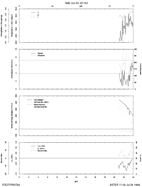
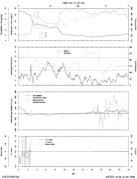
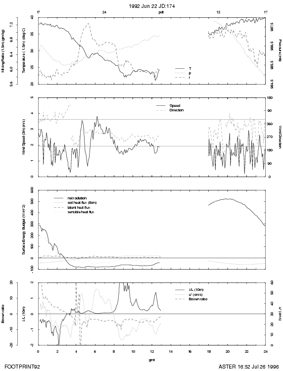
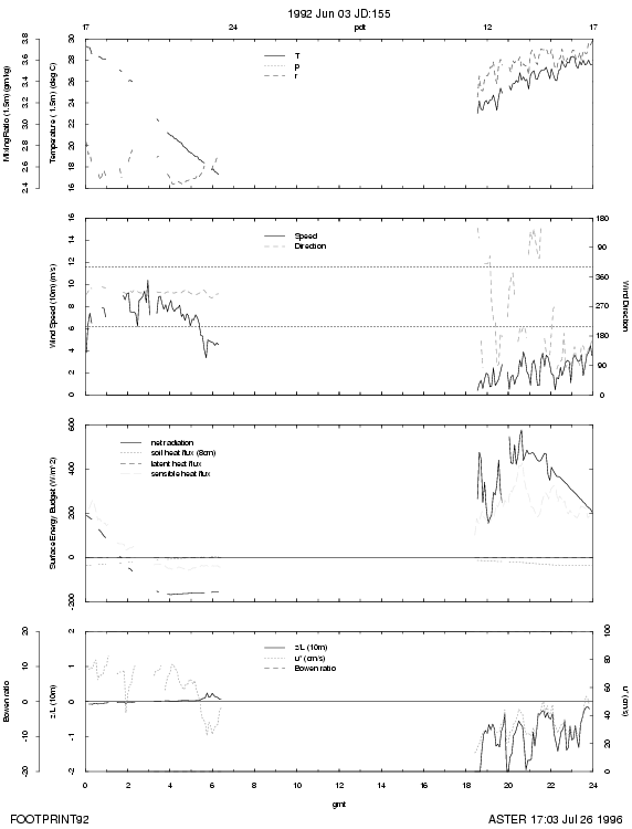
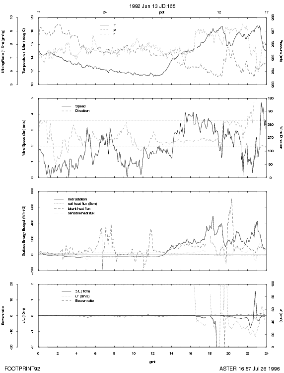
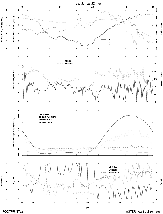
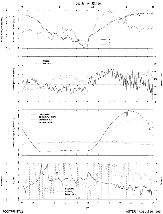
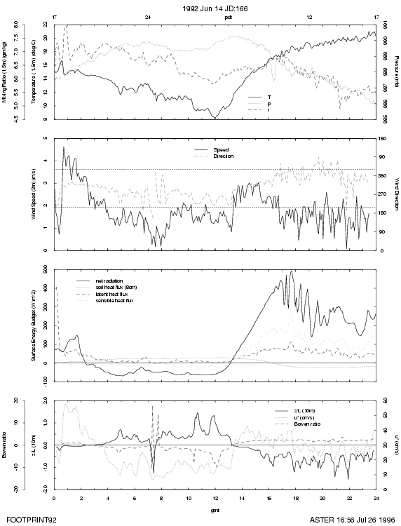
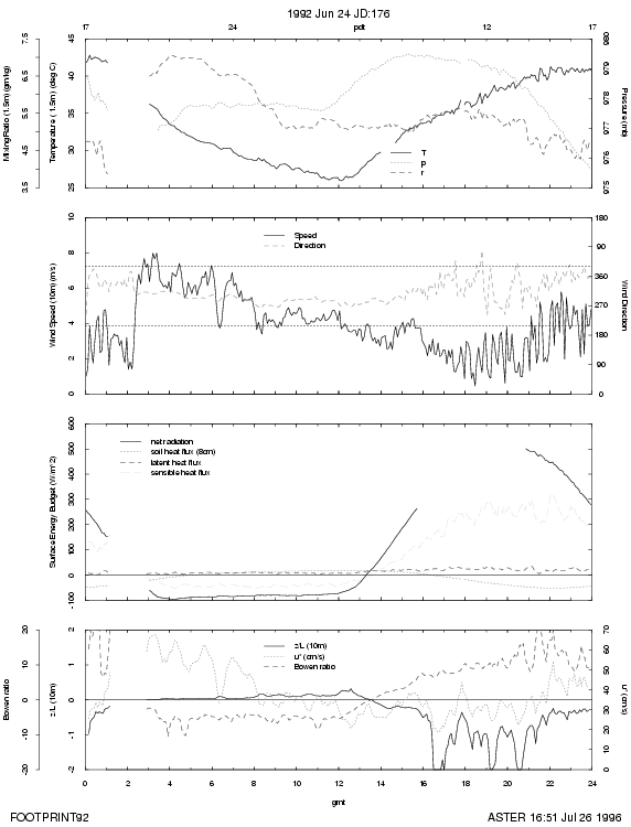
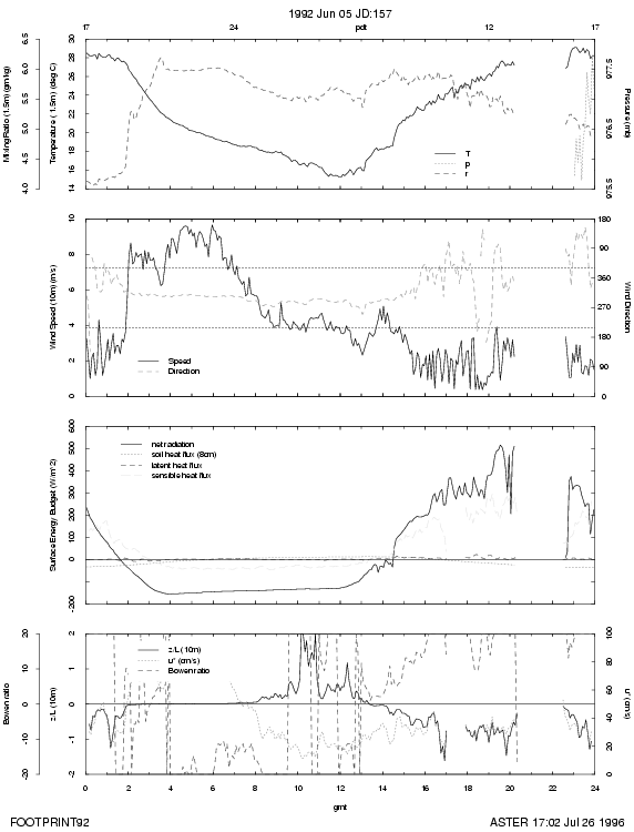
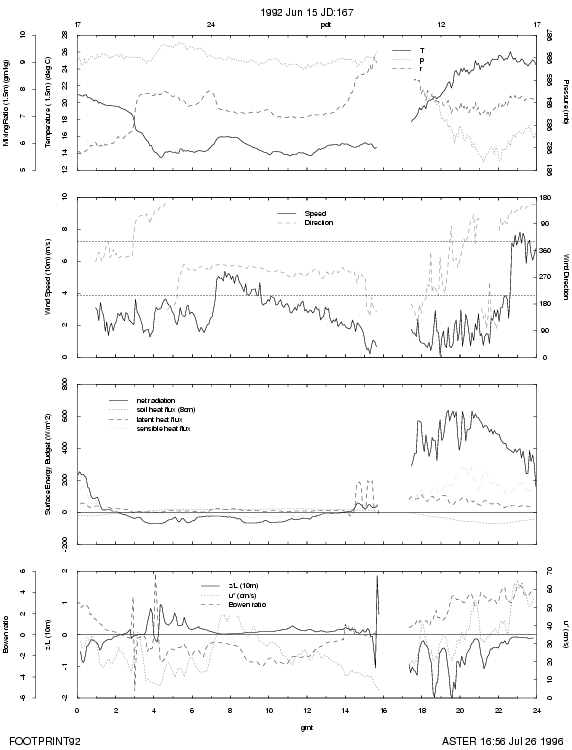
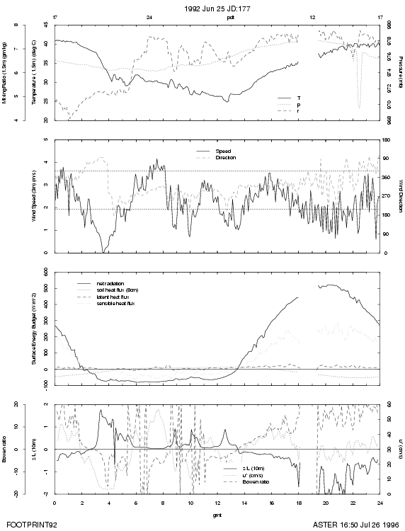
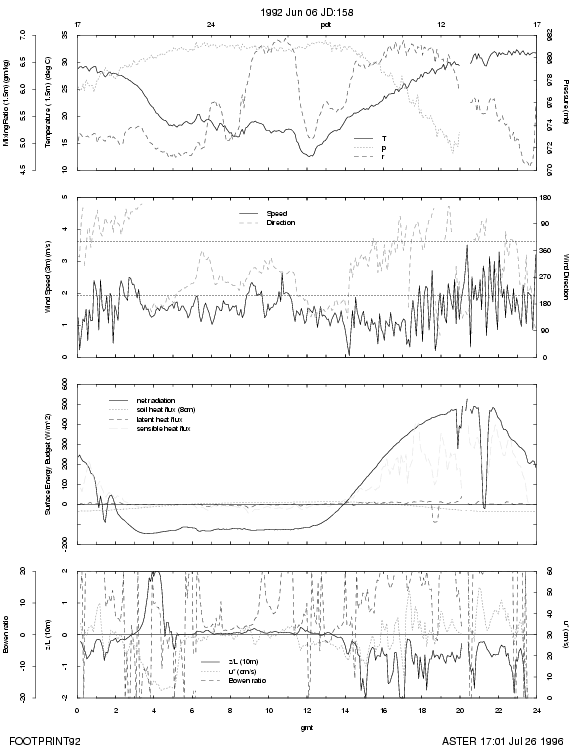
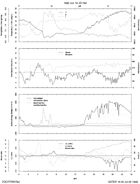
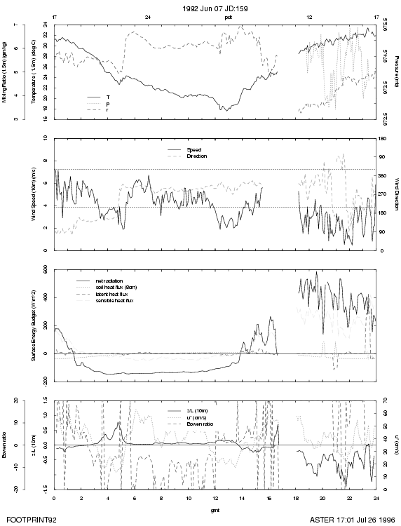
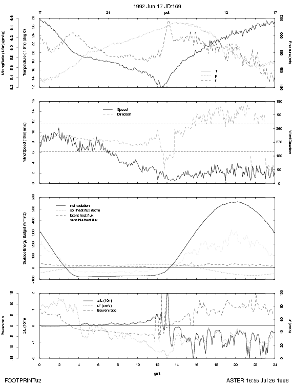
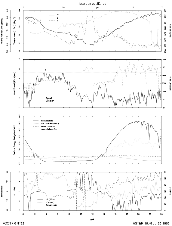
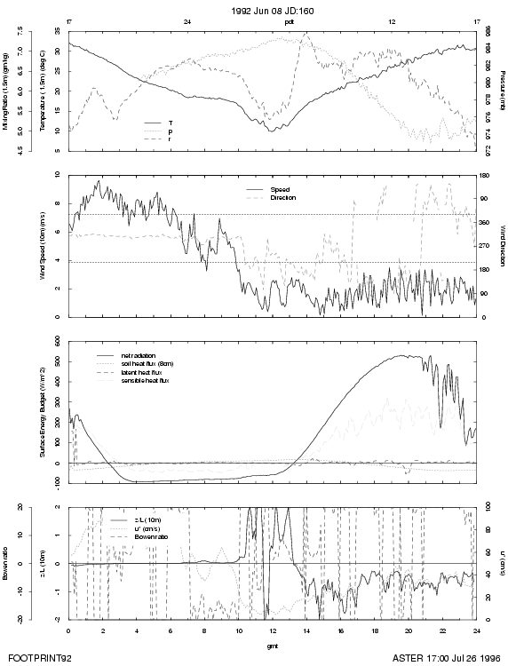
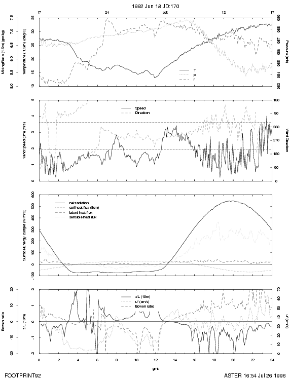
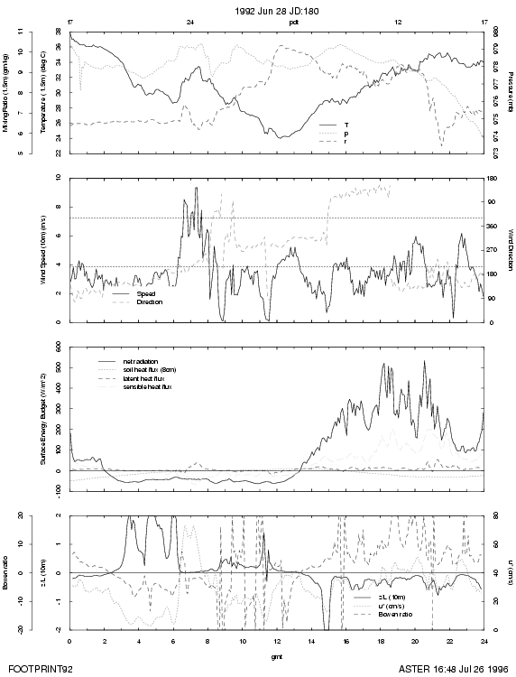
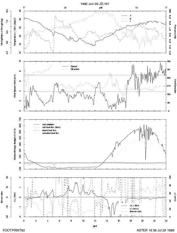
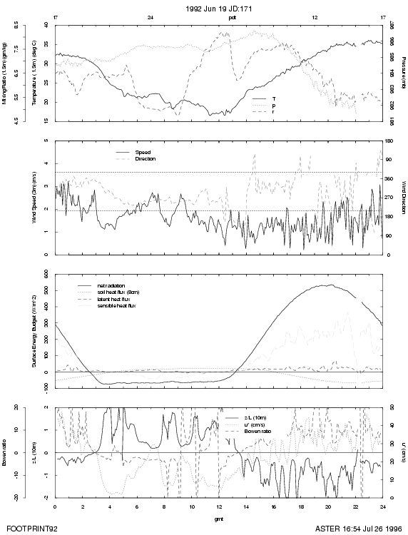
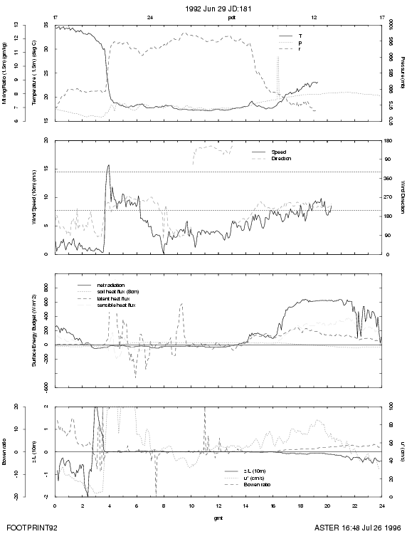
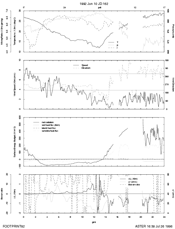
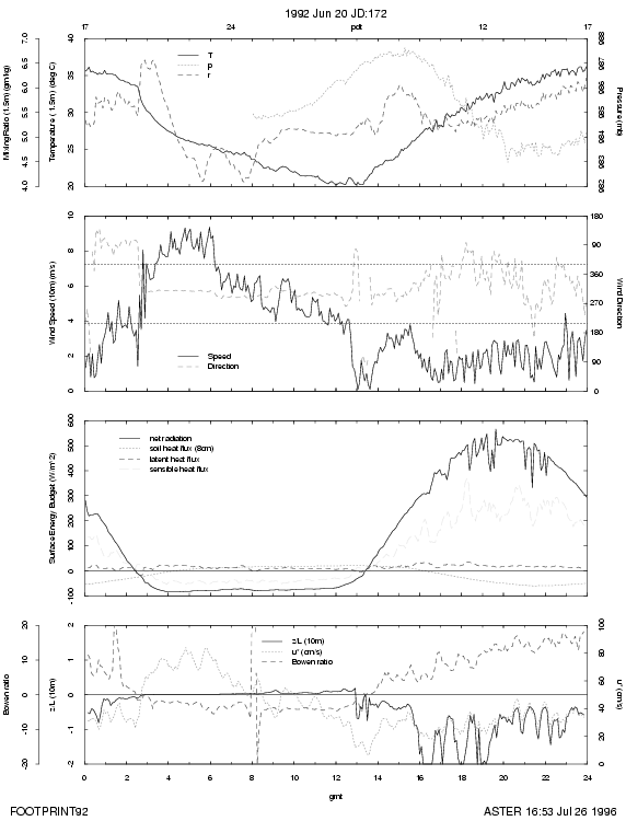
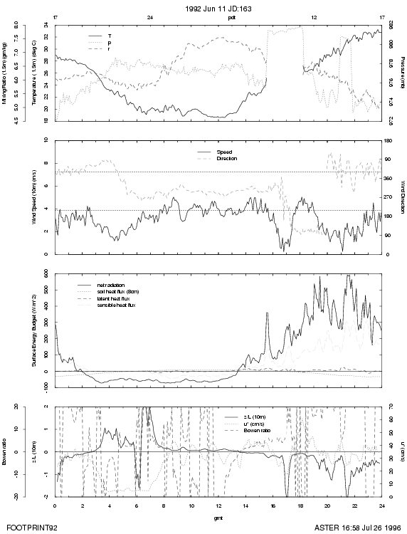
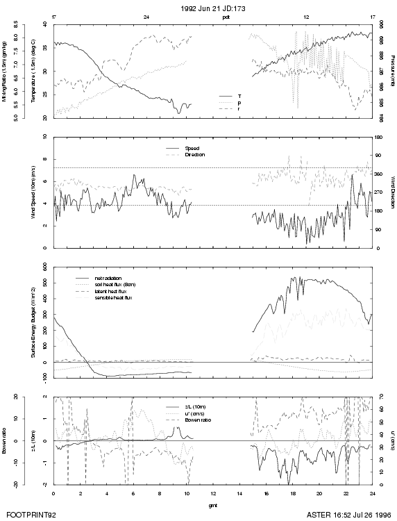
Daily weather plots
A selection of covar plots were produced daily to provide a review of the operations. These are termed "Daily Weather Plots."
The daily weather plots presented in the appendix of this report are:
-
- temperature, humidity, pressure and rainfall
- wind speed and direction
- net radiation, sensible heat flux, latent heat flux, and surface heat flux
- z/L, u* and the Bowen ratio. The plotted data are 5 minute covar plots, except for the turbulent flux data, sensible and latent heat fluxes, z/L, u* and the Bowen ratio, which are 20 minute averages
The plots can be found here.
Wind
The prop-vanes are integrated sensors which yield wind speed and direction directly as a serial output. The prop-vane wind components are output in a geographic coordinate system; where u is wind from the west and v is wind from the south. The propvanes are individually calibrated for wind speed response in the SSSF wind tunnel prior to the deployment.
The sonic anemometers are integrated sensors. The ATI sonic anemometers output the three orthogonal wind components and the derived speed of sound temperature. The UW sonic anemometers measure three non-orthogonal wind components from which the three orthogonal wind components are calculated. In both cases, the wind components are in an instrument-oriented coordinate system, where u is the wind along the instrument boom towards the tower and v is the wind from right to left as you face in the positive u direction. A nominal bearing derived from the azimuth of the mounting boom is used to obtain the approximate geographic wind components during the field program. In post project analysis of the sonic anemometer data, the accurate geographic winds are derived by matching the sonic anemometer data with that of the propvanes.
Psychrometry
The psychrometers are integrated sensors which yield relative humidity and temperature directly as output. From these measured values other moisture parameters can be calculated.The psychrometers are calibrated in the SSSF calibration lab prior to the field program
Radiation
The radiation stand bearing the radiation sensors was positioned over a representative surface with grass, small scrub and a patch of sand. The 3-meter-long horizontal beam of this radiation stand was 3 meters above the ground and oriented nominally east-west (a theodolite sighting indicated the bearing to be 260° 48'). The level-adjustable assembly bearing the radiation sensors was mounted on the beam and leveled to within 15'. Six radiation sensors were deployed: a four component radiation array monitoring incoming and outgoing short and long wave radiation with Eppley radiometers, a REBS net radiometer, and an Everest surface temperature sensor. The two long-wave radiometers and the net radiometer output analog voltages. The short-wave radiometers gave similar signals together with thermistor output defining the temperature of the instruments' case and dome. This enabled a correction to be made to compensate for the direct sunlight heating of the dome of the shortwave sensor.
It is important to appreciate that the short-wave radiometers and the net radiometer view a hemisphere with a cosine weighting factor. For the incoming radiation this presents no difficulty if the sensors are horizontally level. For the outgoing radiation it implies that the effective viewing area of the sensors at 3 meters height is only a few tens of square meters. This constraint puts a premium upon the representativeness of the surface under the radiation stand.
The Everest surface temperature sensor has a collimated 30 degree cone and views a patch of the surface less than ten square meters in area. The sensor yields an output directly in degrees centigrade by using an assumed infrared emissivity of 0.95.
Soil Parameters
Three locations, corresponding to the three dominant surface covers, sagebrush, senescent grass, and bare sand, were instrumented to determine the surface heat flux. At each location four soil temperature probes were inserted at 1 cm, 3cm, 5 cm, and 7 cm depth, and a soil heat flux plate was buried at 8 cm. The output of the four soil temperature probes were connected to the data system via a self timing multiplexer. The multiplexer generated an indicator signal to enable the correct assignment of the different outputs. The temperature profile of the soil and the average temperature of the top 8 cm was determined. Generally, every day or so, the soil moisture for the top 8 cm of soil was determined near mid-day using the gravimetric, dig, cook and weigh method. Soil samples were taken at the three locations and returned to the laboratory for subsequent analysis. The bulk density, the mineral density and an estimate of volumetric organic fraction were determined for the FOOTPRINT92.
-
- bulk density = 1.60 gsoil.cm^-3soil, or 1.60 x 10³ kgsoil.m^-3soil
- mineral density = 2.6 gmineral.cm^-3mineral, or 2.6 X 10³ kgmineral.m^-3mineral
- volumetric organic fraction = 0.01 cm^3organic.cm^-3soil or 0.01 m^3organic.m^-3soil
From these parameters and the gravimetric water fraction the volumetric heat capacity of the soil and hence the heat capacity of the top 8 cm of the soil was determined. From the heat capacity and the varying average temperature the heat stored in the layer of soil above the heat flux plates was calculated. The heat flux measured at the 8 cm depth was subjected to the Phillips correction, to compensate for the effect of the different heat conductivities of the heat flux plate and the soil. The soil heat flux at 8 cm depth taken together with the heat stored in the top 8 cm of soil yield the heat flux at the surface of the soil.
Post Project Analysis of Sonic Anemometer Data
The post-project analysis of the sonic anemometer data to correct for bias and tilt was carried out using the two functions: " fun.sonic.bias.plot" and "fun.sonic.tilt.plot" which were composed by T. Horst and subsequently modified by G. Maclean. These functions are available on request.
Specified values for parameters which were utilized in this analysis were:
-
- prop.corr = 65.75 degrees for ops1
- flagmax = 0.1 for ops1, ops2, and ops3
- wmax = 1.0 ms-1 for ops1, ops2, and ops3
(With the exception of ops2, "atiS.50.10m," 172 to 174 when a value of wmax = 5.0 ms-1 was used)
"prop.corr"
The correction applied to the geographic bearing of the prop-vanes. During ops1 prior to the theodolite sighting, a default bearing of 0 degrees = true north was used in the prop-vane microprocessor. For ops2 and ops3 the true bearing was incorporated in the microprocessor.
"flagmax"
An indication of the extent of sonic anemometer spiking. The sonic anemometer data is despiked using a statistical screening procedure derived by Jorgen Hostrup. (Hostrup, J., 1993, A statistical data screening procedure, Meas. Sci. Technol., 4, 153-157). Individual wind component values lying outside their predicted range are replaced by forecasted values. When the fraction of thus-corrected individual points within a five minute covar interval exceeds the value of flagmax, then the entire five minute covar period is rejected.
"wmax"
The maximum acceptable indicated vertical air motion offset.
Operations: ops1, ops2, and ops3
Three configuration were specified during the FOOTPRINT92 deployment:
- 1) ops1 from jday 154 to 157
-
-
-
- all sonics at 10m height on the four towers
- atiK.50.10m, uw.100.10m, uw.175.10m, atiK.250.10m
- all sonics at 10m height on the four towers
-
-
-
- prop vane at 10 m at 50m station used to define the true wind direction.
- prop vane azimuth not adjusted and a prop vane correction of 65.75 degrees needed
-
-
- 2) ops2 from jday 157 to 174
-
-
-
- all sonics at 10m height on the four towers
- atiK.50.10m, uw.100.10m, uw.175.10m, atiK.250.10m (jday 157:163)
- atiS.50.10m, uw.100.10m, uw.175.10m, atiK.250.10m (jday 167:174)
- all sonics at 10m height on the four towers
-
-
-
- prop-vane at 10 m at 50m station used to define the true wind direction
- prop-vane azimuth correctly entered in microprocessor and no prop vane correction needed
-
-
- 3) ops3 from jday 174 to 181
-
-
-
- all sonics at 5m height on the four towers
- atiK.50.5m, uw.100.5m, uw.175.5m, atiK.250.10m
- all sonics at 5m height on the four towers
-
-
-
-
-
- prop-vane at 5 m at 50m station used to define the true wind direction
- prop-vane azimuth correctly entered in microprocessor and no prop vane correction needed
-
-
Alignment
These routines use linear-regression.
For all sonic anemometers for each ops the sonic anemometer azimuths were determined with a theodolite. These values of sonic.azm are the nominal values. The first step in processing the sonic anemometer data was to determine the true values for sonic.azm. This was done by comparing the difference between the prop-vane and the sonic anemometer as the wind direction varied. The value of the function,
total error = (error in aa + error in v2)0.5
was plotted as a function of the assumed azimuth of the sonic. A minimum in the curve was assumed to correspond to the true azimuth of the sonic anemometer.These true sonic.azm's were then used as input to the bias program which plots u and v wind components as measured by the sonic anemometer and the prop-vane. The gains and intercepts of these lines are given as "u.gain," "v.gain," "u.off," and "v.off."
These gains and intercepts were then used as input to the tilt program, which calculates for each sonic for each ops the offset, pitch and roll.
Table 3 summarizes the sonic anemometer data where:
-
- "sonic.azm" is the true azimuth of the sonic anemometer
- "prop.corr" is the correction applied to the prop-vane azimuth
Sulfur Hexafluoride Releases.
Table 4: Summary of SF6 Release Periods
| Test # | Start | Stop | Duration | Type | NW Winds | Duration |
|---|---|---|---|---|---|---|
| 1 | 154:2106 | 155:0250 | 5:44 | line | 2300-0250 | 3:50 |
| 2 | 156:1754 | 157:0115 | 7:21 | line | 1754-2400 | 6:06 |
| 3 | 157:1327 | 157:1546 | 2:19 | line | 1327-1500 | 1:33 |
| 4 | 158:2048 | 158:2325 | 2:37 | point | ||
| 5 | 159:2021 | 160:0759 | 10:38 | line | 0000-0759 | 7:59 |
| 6 | 160:2350 | 161:0213 | 2:23 | line | ||
| 7 | 161:2001 | 161:2329 | 3:28 | point | ||
| 8 | 161:2342 | 162:1642 | 16:42 | line | 2342-0100 | 1:17 |
| 0330-1130 | 8:00 | |||||
| 9 | 163:1551 | 163:1812 | 2:21 | line | 1551-1700 | 1:09 |
| 10 | 166:1610 | 166:1739 | 1:29 | line | 1610-1630 | 0:20 |
| 11 | 166:1925 | 166:2329 | 4:14 | point | ||
| 12 | 167:0050 | 167:0305 | 2:15 | line | 0050-0250 | 2:00 |
| 13 | 168:1623 | 169:1624 | 24:01 | line | 1623-1200 | 19:37 |
| 1345-1500 | 1:15 | |||||
| 14 | 171:0753 | 171:1810 | 10:37 | line | 0753-1230 | 4:37 |
| 1500-1700 | 2:00 | |||||
| 15 | 172:0731 | 171:1803 | 10:32 | line | 0731-1300 | 5:29 |
| 1400-1600 | 2:00 | |||||
| 16 | 173:0155 | 173:1616 | 14:21 | line | 0155-1616 | 14:21 |
| 17 | 174:0132 | 174:1537 | 14:05 | line | 0430-1200 | 7:30 |
| 18 | 176:0507 | 176:1734 | 12:27 | line | 0507-1700 | 11:53 |
| 19 | 177:0647 | 177:2020 | 13:33 | line | 0647-1930 | 12:43 |
| 20 | 178:0313 | 178:1832 | 15:19 | line | 0313-0800 | 4:47 |
| 1500-1600 | 1:00 | |||||
| 21 | 179:0232 | 179:1806 | 15:34 | line | 1200-1600 | 4:00 |
| 0232-0800 | 5:28 | |||||
| 22 | 180:0344 | 180:1723 | 13:39 | line | 0930-1500 | 5:30 |
| 23 | 181:0343 | 181:1618 | 14:35 | line | 0400-0700 | 3:00 |
| Totals: | 219:54 | 137:24 |
Appendix
Available Covars
The set of covar parameters immediately available is listed in Table 5. Other parameters can be calculated.
N.B. covariances are shown in the form "w:t.100.5m" where this implies "w.100.10m:t.100.10m."
Daily Weather Plots
The daily weather plots presented in the appendix are:
-
- temperature, humidity, pressure and rainfall
- wind speed and direction
- net radiation, sensible heat flux, latent heat flux, and surface heat flux
- z/L, u*
The values plotted for temperature, humidity, pressure, rainfall, wind speed and direction, net radiation and surface heat flux are 5 minute averages, while the values plotted for the sensible heat flux, the latent heat flux, Z/L and u* are 20 minute averages.
The plots are listed according to Julian day:
| 154 | 164 | 174 |
| 155 | 165 | 175 |
| 156 | 166 | 176 |
| 157 | 167 | 177 |
| 158 | 168 | 178 |
| 159 | 169 | 179 |
| 160 | 170 | 180 |
| 161 | 171 | 181 |
| 162 | 172 | |
| 163 | 173 |
Field Logbook
An electronic logbook was maintained during the field program. A total of ~170 entries were made during the FOOTPRINT92 deployment in 17 different categories.


