CHATS
Canopy Horizontal Array Turbulence Study
![]() Logo by Lori Mattina
Logo by Lori Mattina
Introduction
This document describes the operation and measurements of the Integrated Surface Flux System (ISFS) during the Canopy Horizontal Array Turbulence Study field experiment (CHATS), March 15th to June 15th, 2007.
The objective of CHATS was to make spatial measurements of the velocity and scalar turbulence fields in a uniformly vegetated canopy, using arrays of sonic anemometer/thermometers augmented with fast response water vapor and carbon dioxide sensors. With this spatial information, the three-dimensional fields of velocity and scalar fluctuations can be studied to quantify turbulence transport processes and coherent structures throughout the canopy layer. An ancillary goal was to characterize the turbulent structure of the fields of wind, temperature, humidity, and trace chemical species within and above the orchard canopy.
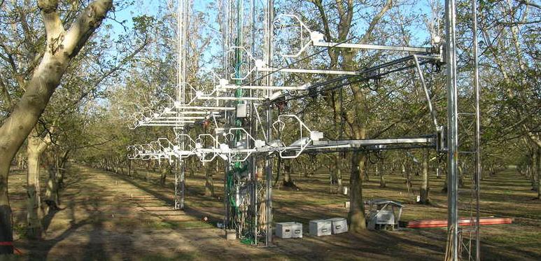
18 sonic anemometers were deployed in a two-level, horizontal array, which had 9 sonics on each of two horizontal beams with a vertical separation of 1 m. The two horizontal beams were supported by 4 towers which are 9 m tall, and the horizontal length of this array was 15-16 m. The sonics were augmented with 5 Campbell KH2O and 5 Li-Cor LI-7500 fast-response water vapor and carbon dioxide sensors, as well as 5 vertical hot-film anemometers. The dimensions of the array (height and sonic spacing) were changed roughly once per week to obtain data within a range of those dimensions and canopy density.
The main sonic array was supplemented with a 30 meter vertical profile of 13 sonic anemometers and 12 hygrothermometers, extending from near the surface, through the canopy and roughness sublayer, to well above canopy top. Also requested are fast-response static pressure sensors and hot-wire/film anemometers to be collocated with the sonic anemometers in the horizontal array, as well as a digital camera system to measure leaf area index (LAI). Finally radiation and soil measurements were made to complete the thermal energy budget of the canopy.
Measurement Sites
The ISFF measurements were made in the Cilker Chandler walnut orchard in the quarter section southwest of the intersection of Sievers and Pitt School Roads near Dixon, CA. ISFF instrumentation was centered on the 59th N/S row of trees west of Pitt School Road. The 30 m tower was located roughly 123 m south of the north edge of the orchard and the horizontal array was located roughly 239 m south of the north edge.
Also located nearby was an NCAR sodar/RASS system and the NCAR REAL scanning lidar. REAL was located north of Sievers Road in order to scan south over the orchard with vertical scans centered between N/S orchard rows 60 and 61 west of Pitt School Road.
Instrumentation
The following table shows the instrument heights and spacing for the 6 different configurations of the horizontal array: 3 array heights at 2 different instrument spacings.
| sensor | heights (nominal) |
horizontal spacing | variables | orientation |
|---|---|---|---|---|
| 9 CSAT3 sonic anemometers top beam |
10.6 m 5.9 m 3.0m |
0.5 m 1.72 m |
(u, v, w, tc).(1-9)t.?m.ha | south |
| 5 CSI krypton hygrometers, top beam |
10.6 m 5.9 m 3.0 m |
0.5 m 1.72 m |
(kh2oV, kh2o).(3-7)t.?m.ha | vertical (footnote A) |
| 5 Dantek hot-film anemometers, top beam |
10.6 m 5.9 m 3.0 m |
0.5 m 1.72 m |
va.(3-7)t.?m.ha | south |
| 9 CSAT3 sonics bottom beam |
9.6 m 4.9 m 2.0 m |
0.5 m 1.72 m |
(u, v, w, tc).(1-9)b.?m.ha | south |
| 5 Licor 7500's, bottom beam |
9.6 m 4.9 m 2.0 m |
0.5 m 1.72 m |
(h2o, co2).(3-7)b.?m.ha | (footnote B) |
| NCAR TRH hygro-thermometers, top |
10.6 m 5.9 m 3.0 m |
central tower; inlet at exact sonic ht |
(T, RH).t.?m.ha | ~southeast |
| NCAR TRH hygro-thermometer, bottom |
9.6 m 4.9 m 2.0 m |
central tower; inlet at exact sonic ht |
(T, RH).b.?m.ha | ~southeast |
| Garmin GPS 35 | NA | (lat, lon, alt).ha | NA |
| sensor | heights/depths (preliminary) |
variables | orientation |
|---|---|---|---|
| 13 CSAT3 sonics | 1.5 3 4.5 6 7.5 9 10 11 12.5 14 18 23 29 m | (u,v,w,tc).?m.vt | west |
| 6 CSI krypton hygrometers | 1.5 4.5 7.5 10 14 23 m | (kh2oV,kh2o).?m.vt | vertical (footnote A) |
| 3 Dantek triple hot-film anemometers | 6 10 14 m | v(a,b,c).?m.vt | south |
| 12 NCAR TRH hygro-thermometers | 1.5 3 4.5 6 7.5 9 10 11 14 18 23 29 m | (T,RH).?m.vt | east; below canopy & 29 m: inlets at sonic ht |
| 2 fast pressure | w/ sonic, both at 1m above canopy | p.(usfs,ncar).11m.vt | NA |
| Paroscientific barometer | 1 m | (P,etc).paro.1m.vt | NA |
| Pyranometer, Epply | 2 m | Rsw.in.vt Rsw.out.vt |
up & down |
| Pyrgeometer, Epply | 2 m |
(Rpile,Tcase,Tdome).in.vt (Rpile,Tcase,Tdome).out.vt |
up & down |
| Pyranometer, Kipp&Zonen | 16 m |
Rsw.in.16m.vt Rsw.out.16m.vt |
up & down |
| Pyrgeometer, Kipp&Zonen | 16 m | (Rpile,Tcase).in.16m.vt (Rpile,Tcase).out.16m.vt |
up & down |
| 4 LI-190SA PAR sensors | ?? m | Rpar.in.?m Rpar.out.?m |
up & down |
| K&Z large-aperture scintillometer | 10 m | data not ingested by ISFF | south |
| ACD REA aerosol sampler | 14 m | ? | west |
| REBS soil temperature | 5 cm | Tsoil.vt | near rad stand |
| Decagon Ech2o soil moisture | 5 cm | Qsoil.vt | near rad stand |
| REBS HFT-3 soil heat flux | 5 cm | Gsoil.vt | near rad stand |
| Hukseflux TP01 thermal properties | 5 cm | (Vpile,Vheat,Tau63).vt | near rad stand |
| Tipping bucket rain gauge | 1 m | rain | near rad stand |
| Garmin GPS 35 | (lat,lon,alt) | NA |
| sonic spacing (m) |
sonic heights (m, nominal) |
start (PDT) |
end (PDT) |
good wind dir (hr) |
hot films single / triple |
|---|---|---|---|---|---|
| 0.5 m | 9.6, 10.6 | Mar 13 17:00 | Mar 22 11:40 | 56:25 | no |
| 0.5 m | 9.6, 10.6 | Mar 22 16:05 | Mar 23 15:05 | 3:50 | no |
| 0.5 m | 4.9, 5.9 | Mar 23 15:35 | Mar 27 14:40 | 43:05 | no |
| 0.5 m | 2.0, 3.0 | Mar 27 14:50 | Mar 31 10:00 | 11:40 | no |
| 1.72 m | 9.6, 10.6 | Mar 31 20:00 | Apr 4 10:55 | 35:55 | Apr 1 12:40 |
| 1.72 m | 4.9, 5.9 | Apr 4 17:15 | Apr 6 15:30 | 17:10 | yes |
| 1.72 m | 4.9, 5.9 | Apr 6 17:00 | Apr 8 14:30 | 29:30 | no |
| 1.72 m | 2.0, 3.0 | Apr 8 17:25 | Apr 15 12:30 | 30:55 | yes |
| 1.72 m | 9.6, 10.6 | Apr 15 17:10 | May 10 16:00 | 196:55 | no |
| 1.72 m | 9.6, 10.6 | May 10 18:30 | May 17 9:09 | 90:10 | 11 May 12:18 to 17 May 09:08 singles 140 hrs triples 74 hrs |
| 1.72 m | 4.9, 5.9 | May 17 13:47 | May 25 15:50 down 2hr 5/23 |
49:25 | 17 May 14:03 to 23 May 16:13 singles 127 hrs triples 138 hrs |
| 1.72 m | 2.0, 3.0 | May 25 19:05 | May 29 9:09 | 23:15 | singles >26? hrs triples 9? hrs |
| 0.5 m | 9.6, 10.6 | May 29 16:50 | June 2 9:10 | 57:20 | yes |
| 0.5 m | 4.9, 5.9 | June 2 10:15 | June 6 9:15 | 48:45 | yes |
| 0.5 m | 2.0, 3.0 | June 6 10:00 | June 11 7:30 | 41:35 | yes |
Good wind direction hours are determined from the medians of the wind directions from the upper 9 sonics in each configuration.
Good direction hours are the sum of continuous periods of 20 minutes or more with directions within ±30° of south.
Times in sixth column are start times for hot film data ingest if different from column 3.
Sensor Notes
Sonic Anemometers
The CHATS sonic anemometers were deployed in two locations. On the vertical profile tower (vt), they were mounted on the south face of the 30 m tower, with the booms pointing to the west, and in the horizontal arrays (ha) the booms were pointed to the south. The horizontal arrays consisted of two levels of 9 sonics each with heights separated by 1 m. The horizontal array sonics were numbered 1-9 from west to east and the two levels were designated as (b)ottom and (t)op.
The CSAT sonic anemometers were tested in the EOL wind tunnel both prior to and following the field program. Sonics that had offsets prior to the field project that exceeded the manufacturer's specification of 4 cm/s were sent back to Campbell Scientific for recalibration. Following the field project, several sonics had offsets ranging from 6 to 15 cm/s. For those sonics, the following table lists the offsets to the orthogonal wind components, u, v, w, as well as the offsets to the measured, non-orthogonal components, a, b, c. Note that in most cases, only one of the measured wind components exceeds the manufacturer's specification, but that this can adversely affect more than one of the orthogonal wind components.
| S/N | location | u (cm/s) | v (cm/s) | w (cm/s) | a (cm/s) | b (cm/s) | c (cm/s) |
|---|---|---|---|---|---|---|---|
| 0673 | 1.5m vt | 2 | -9 | -1 | -1 | -4 | 4 |
| 0674 | 3m vt | 4 | -15 | -4 | -6 | -9 | 3 |
| 0540 | 7.5m vt | -3 | 8 | -4 | -2 | -1 | -8 |
| 0536 | 9m vt | 6 | -8 | 2 | -2 | 0 | 7 |
| 0671 | 10m vt | -9 | 8 | -7 | -2 | -5 | -11 |
| 0743 | 12.5m vt | 0 | -7 | -2 | -2 | -5 | 1 |
| 1123 | 14m vt | 9 | 3 | -2 | -7 | 2 | -1 |
| 0744 | 29m vt | 6 | -6 | 0 | -3 | -1 | 4 |
| 0672 | 2b ha | -11 | -2 | 2 | 7 | -2 | 0 |
| 0855 | 3b ha | 12 | 7 | 5 | -2 | 10 | 5 |
| 0366 | 5b ha | 14 | 13 | 1 | -6 | 10 | -1 |
| 0378 | 6b ha | -4 | -7 | 4 | 5 | -1 | 5 |
| 0677 | 7b ha | 3 | -8 | -1 | -2 | -3 | 4 |
| 0376 | 8b ha | -5 | 6 | -3 | 0 | -1 | -7 |
| 1119 | 5t ha | -7 | 7 | -3 | 1 | -1 | -8 |
| 0539 | 8t ha | -10 | 9 | -2 | 3 | 0 | -8 |
Following the project, the sonic tilts were calculated with the planar fit technique, using the 5-minute-averaged wind components. This process was applied to each period for which the mounting of a sonic was unchanged. The sonic tilt angles were then used to rotate the sonic data into a flow-parallel coordinate system with a time-averaged vertical velocity of zero. For the vertical profile tower, the U wind component is positive from west to east and the V component is positive from south to north. For the horizontal array, the U wind component is normal to the array and positive from south to north, and the V component is parallel to the array and positive from east to west.
For CHATS, we restricted the data used for the tilt calculations to nighttime data, since the daytime data appeared to be noisier presumably due to sweeps and ejections from the overlying flow into and out of the canopy. For this purpose, we used the incoming shortwave radiation at 16 m to separate daytime from nighttime. For the profile tower we also eliminated data with wind directions within ±45° from the direction of the tower, i.e. into the 'back' of the sonic. For the sonics on the horizontal array, we only accepted wind directions within ±60° from parallel to the sonic U axis, i.e. into the 'front' of the sonic.
For the most part, the sonics on the profile tower were fixed in place for the duration of the project. There were two exceptions. First the original sonic at 6m (S/N 0740) was unable to operate at 60 Hz and was replaced with S/N 1119 on the morning of March 22nd, apparently around 10 am. The second exception was that the height of the 14m sonic was changed from 14.09 m to 14.52 m around 5 pm March 25th in order to allow raising of the boom to service one of the hot film anemometers. Above 10 m, data from the entire project were used to determine the sonic tilt angles. Below 10 m, data were used only until leaf-out in mid to late April, and it was assumed that the derived tilt angles applied for the entire project. Among other things, the tilt calculations within and below the canopy after leaf-out exhibited unrealistic vertical velocity offsets. Another difficulty with these data is the lack of data above 1 m/s, a threshold used in the tilt calculation to minimize the occurance of turbulent gusts with large wind elevation angles.
| Sonic | 1.5m | 3m | 4.5m | 6m | 7.5m | 9m | 10m | 11m | 12.5m | 14m | 18m | 23m | 29m |
|---|---|---|---|---|---|---|---|---|---|---|---|---|---|
| w offset (cm/s) |
0 | 0 | -2 | -3 | -2 | -4 | -6* | -1* | -3* | -1 | 0 | 0 | 2 |
| lean (deg) |
0.9 | 2.2 | 2.6 | 3.0 | 2.4 | 1.0 | 2.0 | 1.4 | 1.2 | 1.3 | 1.6 | 1.3 | 1.5 |
| lean azimuth (deg) |
37.2 | 47.5 | 27.7 | 25.6 | 6.7 | 12.8 | 21.8 | 27.1 | 75.8 | 19.0 | 47.1 | 57.7 | 61.0 |
In contrast, the configuration of the horizontal array sonics was changed multiple times during the project. Each configuration is characterized by a sonic spacing and the heights of the two linear arrays. The sonic spacing was changed twice during the project, once on March 31st from 0.5 m to 1.72 m and again on May 29th from 1.72 m back to 0.5 m. For each sonic spacing, the array was moved to three different heights by raising and lowering the horizontal ASTER towers supporting the two levels of sonics. With two exceptions, the sonic mountings were not changed during the raising and lowering of the linear arrays, and thus a single tilt fit can be calculated for each of the three periods with a constant sonic spacing.
Both exceptions are associated with the 1.72 m sonic spacing. Each of the two levels of these arrays consisted of 4 sonics mounted on each of two horizontal ASTER tower sections, e.g. sonics 1b-4b on the west and 6b-9b on the east, plus a fifth sonic, 5b in the lower array and 5t in the upper array, mounted on a vertical Rohn tower placed between the west and east halves of the wide arrays. Thus the mounting of sonics 5b and 5t was changed every time the height of the array was changed and a separate tilt fit calculation is necessary for each height.
The second exception occurred on April 15th, when the EMT tubing used to provide additional support between the individual sonics was stiffened by inserting wooden dowels at the junctions between the tubing. This was done for the upper and lower east arrays, but only for the upper west array. Thus sonic tilts were calculated separately for the periods before and after April 15th.
| Sonic | 1b | 2b | 3b | 4b | 5b | 6b | 7b | 8b | 9b |
|---|---|---|---|---|---|---|---|---|---|
| w offset (cm/s) |
3 | 1 | 2 | 2 | 2 | 3 | 0 | 3 | -1 |
| lean (deg) |
4.2 | 4.2 | 5.1 | 5.5 | 5.2 | 5.6 | 5.8 | 6.4 | 5.4 |
| lean azimuth (deg) |
3.8 | 2.1 | -8.7 | -8.0 | -6.0 | -10.7 | -7.5 | -7.8 | -3.8 |
| Sonic | 1t | 2t | 3t | 4t | 5t | 6t | 7t | 8t | 9t |
| w offset (cm/s) |
2 | 2 | 1 | 1 | 0 | 0 | 2 | 1 | 0 |
| lean (deg) |
3.3 | 2.5 | 3.0 | 3.3 | 3.0 | 3.3 | 3.6 | 3.6 | 3.6 |
| lean azimuth (deg) |
17.1 | 21.3 | 11.2 | 3.0 | -2.7 | -3.6 | -11.6 | -24.9 | -23.7 |
| Sonic | 1b | 2b | 3b | 4b | 5b 9.63m |
5b 4.95m |
5b 2.00m |
6b | 7b | 8b | 9b |
|---|---|---|---|---|---|---|---|---|---|---|---|
| w offset (cm/s) |
4 | 2 | 3 | 3 | 4 | 2* | NA | 3 | 2 | 2 | -1 |
| lean (deg) |
3.7 | 3.4 | 4.6 | 5.3 | 4.2 | 3.2 | NA | 3.1 | 4.9 | 4.5 | 3.7 |
| lean azimuth (deg) |
-1.6 | -6.3 | -5.1 | -0.8 | 4.3 | 4.0 | NA | -2.6 | 3.2 | -0.2 | -5.9 |
| Sonic | 1t | 2t | 3t | 4t | 5t 10.63m |
5t 5.91m |
5t 2.96m |
6t | 7t | 8t | 9t |
| w offset (cm/s) |
3 | 1 | 1 | 0 | 1 | 1* | NA | 0 | 3 | 1 | -1 |
| lean (deg) |
3.3 | 2.1 | 3.2 | 2.8 | 1.8 | 3.0 | NA | 2.3 | 2.5 | 2.0 | 2.2 |
| lean azimuth (deg) |
-34.9 | 28.0 | 14.7 | -4.5 | 22.1 | -1.4 | NA | 20.3 | 6.8 | -22.5 | -2.5 |
| Sonic | 1b | 2b | 3b | 4b | 5b 9.63 m |
5b 4.95 m |
5b 2.00 m |
6b | 7b | 8b | 9b |
|---|---|---|---|---|---|---|---|---|---|---|---|
| w offset (cm/s) |
4* | 2* | 0 | 2* | 1* | NA | NA | 1 | -1 | 2 | 0* |
| lean (deg) |
6.4 | 5.0 | 5.5 | 7.4 | 4.5 | NA | NA | 5.6 | 6.1 | 7.3 | 4.8 |
| lean azimuth (deg) |
13.7 | -3.5 | 6.5 | -6.6 | 13.1 | NA | NA | 24.3 | 6.1 | -53.4 | 4.3 |
| Sonic | 1t | 2t | 3t | 4t | 5t 10.63 m |
5t 5.91 m |
5t 2.96 m |
6t | 7t | 8t | 9t |
| w offset (cm/s) |
0 | -1 | -1 | -1 | 1* | NA | NA | -2 | -1 | -1 | 0 |
| lean (deg) |
3.7 | 3.8 | 3.9 | 4.1 | 3.8 | NA | NA | 3.7 | 3.0 | 3.0 | 4.3 |
| lean azimuth (deg) |
8.2 | 11.0 | 12.0 | 8.7 | 2.0 | NA | NA | 13.5 | 6.9 | -8.5 | 1.4 |
| Sonic | 1b | 2b | 3b | 4b | 5b | 6b | 7b | 8b | 9b |
|---|---|---|---|---|---|---|---|---|---|
| w offset (cm/s) |
4* | 2* | 0* | 2* | 1* | 2* | 0* | 2* | 0* |
| lean (deg) |
6.8 | 7.3 | 5.9 | 7.8 | 6.8 | 7.0 | 8.2 | 9.8 | 9.4 |
| lean azimuth (deg) |
8.0 | 5.1 | -2.5 | -6.6 | -10.4 | -5.6 | -7.0 | -2.4 | 0.2 |
| Sonic | 1t | 2t | 3t | 4t | 5t | 6t | 7t | 8t | 9t |
| w offset (cm/s) |
0* | 0* | 0* | 0* | 0* | -2* | -1* | 0* | 0* |
| lean (deg) |
4.7 | 5.1 | 4.8 | 4.8 | 5.3 | 4.6 | 4.2 | 5.2 | 5.2 |
| lean azimuth (deg) |
15.4 | 3.0 | 8.5 | -3.7 | -13.7 | -7.5 | -12.1 | -15.1 | -11.1 |
Due to the difficulties after leaf-out mentioned previously, the tilt fits after leaf-out were essentially determined from data at the 9.6 m and 10.6 m heights and assumed to apply to the lower heights for the same sonic spacing. For the same reasons, tilt fits were not possible after April 15th for the 5b and 5t sonics in the wide array at the lower heights. Further, the data at 9.6 m and 10.6 m was often scarce and consequently the raw fits gave unrealistic values for the vertical velocity offset. In those cases, the offset was specified from earlier fits of the same sonic calculated with more extensive data.
The sonic orientations or azimuths were measured with a digital sighting compass known as a DataScope. The largest uncertainty in this technique is identifying the features of the sonic that indicate proper alignment of the DataScope with the sonic U axis. Due to poor sight lines through the trees, this was not done for the sonics above 9 m on the profile tower. The average of the good readings below 9 m, 185.4°, was used for all the unmeasured azimuths.
The sonic azimuths were measured for the horizontal arrays when they were below the canopy at the lowest height, and it was assumed that the azimuths were unchanged as the arrays were raised and lowered. Note that the azimuths for the wide arrays were measured only once, prior to inserting the wooden dowels in the EMT tubing on April 15th. Further, the azimuths of sonics 5b and 5t were also only measured this one time, despite moving those sonics to different heights as the wide configuration was changed. In both latter cases, the measured azimuths were assumed to apply during the unmeasured periods.
The absolute values of the sonic temperatures, tc, are inaccurate by perhaps 1-2 °C because of the inability to maintain the sonic path lengths to a sufficient tolerance. Campbell testing and analyses shows that they can hold CSAT path lengths to better than 0.3 mm out of 11.55 cm, or about 0.26 percent. This gives a 0.26 percent error in the speed of sound, which in turn, gives a sonic temperature error of about 0.52 percent. At 300 K, this is a 1.6 °C error (Note that the wind and temperature fluctuations in this example are in error by only a fraction of one percent).
For this reason, we have calibrated the sonic temperature measurements with a linear fit relative to NCAR hygrothermometers mounted nearby,
tccalibrated = offset + gain * tcmeasured
The temperature and humidity sensors in the NCAR hygrothermometers have been calibrated in the laboratory with respect to NIST-traceable standards. The following tables list the offset and gain applied to sonic temperature measured by each individual sonic. The rms deviations from these fits are on the order of 0.14 °C. The general pattern of these deviations follows a 24-hour cycle that suggests they are associated with residual radiation errors in the hygrothermometer mechanically-aspirated shield.
| sonic | 1b | 2b | 3b | 4b | 5b | 6b | 7b | 8b | 9b | |
| s/n | 0367 | 0672 | 0855 | 0538 | 0366 | 0378 | 0677 | 0376 | 0121 | |
| offset (ºC) | 0.801 | 0.848 | 0.974 | 0.983 | 1.253 | 0.568 | 0.884 | 0.653 | 0.375 | |
| gain | 1.003 | 1.013 | 1.006 | 1.010 | 1.011 | 1.005 | 1.017 | 1.001 | 1.035 | |
| sonic | 1t | 2t.a* | 2t.b* | 3t | 4t | 5t | 6t | 7t | 8t | 9t |
| s/n | 0377 | 0853 | 0120 | 0537 | 1124 | 1119 | 0800 | 1121 | 0539 | 0247 |
| offset (ºC) | 0.720 | 1.013 | 0.413 | 0.934 | 0.887 | 1.049 | 1.079 | 0.693 | 1.137 | 0.873 |
| gain | 1.009 | 1.012 | 1.040 | 1.006 | 1.023 | 1.016 | 1.022 | 1.005 | 1.015 | 1.009 |
| sonic | 1.5 m | 3.0 m | 4.5 m | 6 m | 7.5 m | 9 m | 10m | |||
| s/n | 0673 | 0674 | 1120 | 0119 | 0540 | 0536 | 0671 | |||
| offset (ºC) | 0.681 | 1.069 | 0.816 | 0.316 | 1.070 | 0.440 | 0.855 | |||
| gain | 0.998 | 1.012 | 1.013 | 1.018 | 1.017 | 1.009 | 1.017 | |||
| sonic | 11 m | 12.5 m | 14 m | 18 m | 23 m | 29 m | ||||
| s/n | 0364 | 0743 | 1123 | 0738 | 1117 | 0744 | ||||
| offset (ºC) | 0.712 | 0.451 | 0.773 | 0.407 | 0.894 | -0.295 | ||||
| gain | 1.001 | 1.038 | 1.005 | 1.021 | 1.018 | 1.030 |
Krypton Hygrometers
For application of the flux corrections, here are the coefficients for each krypton hygrometer. Note that all pathlengths were close to 1.3 cm, so Ko = -3.4E-3 m^3/g-cm. "S" is the separation distance from the sonic anemometer. Note that the Kw values used for the last version of NetCDF files were rounded to only 2 digits (e.g. -0.15). Thus, these values could be in error by up to 3%. This will be corrected in the next version of these files.
| position | sensor s/n | x (cm) | Kw | Vo (mV) | S (cm) |
| 23 m | 1525 | 1.36 | -0.148 | 3808 | 22 |
| 14 m |
1393 1397 (after May 21 14:20 PST) |
1.23 1.24 |
-0.150 -0.148 |
4748 4162 |
22 22 |
| 10 m | 1101 | 1.30 | -0.147 | 4786 | 22 |
| 7.5 m | 1394 | 1.20 | -0.152 | 4811 | 22 |
| 4.5 m | 1390 | 1.40 | -0.148 | 5309 | 22 |
| 1.5 m |
1395 1393 (after Jun 8 16:30 PST) |
1.20 1.23 |
-0.143 -0.150 |
3024 4748 |
22 22 |
| 7t | 1258 | 1.35 | -0.150 | 5337 | 22 |
| 6t | 1391 | 1.21 | -0.146 | 3586 | 22 |
| 5t | 1389 | 1.28 | -0.150 | 5158 | 22 |
| 4t | 1392 | 1.20 | -0.150 | 5072 | 22 |
| 3t | 1133 | 1.22 | -0.153 | 5158 | 22 |
CO2 Sensors
Five Li7500s were used in the middle positions on the bottom of the horizontal array to measure co2 and h2o. We have done basic QC by removing data during moves between the array positions and removing data when the sensors were wet. Manufacturer's calibrations were used, which should be reasonable for at least 4 of the sensors since they were purchased new for this project.
Hot-Film Anemometers
Two types of hot-film anemometers were deployed during CHATS. All were intended to measure high-frequency (small-scale) velocity fluctuations that are filtered by the size of the sonic anemometers. Five single-film probes (Dantec 55R11, each using a 54T30 CTA bridge) were oriented vertically at the positions 3t, 4t, 5t, 6t, and 7t on the horizontal array. In addition, triple-film probes (Dantec 55R95?, also using 54T30 CTAs) were placed at heights of 6, 10, and 14 m on the vertical tower. Due to delayed testing in the lab, the probes were deployed about 3 weeks into Phase I, with a test deployment of the vt sensors on March 26th. Real deployment of the vt sensors started March 30th, and of the ha sensors on April 1st. All probes were protected (either covered or removed) during irrigation periods to avoid damage by water spray and removed during the break between Phase I and II.
The sampling rate for each of the channels was 2000 samples/s which was expected to capture scales through the inertial subrange, including the Kolmogorov frequency. Data were archived locally by each data system onto USB disks and manually copied to the base computer every week or so. During Phase I, an error in the data system caused the position of the channels in the data archive to shift over time. To test this problem, a 6th channel with zero Volts was added on about April 9th. By the end of Phase I, this problem appears to have been fixed. More documentation of this problem will be forthcoming to determine how much of the Phase I data are recoverable. During Phase II, the hot-film data acquisition appears to have functioned normally.
The single-film probe at 3t never functioned properly, though its voltage output was similar enough to a normal probe that this problem was not noticed in the field. The probe at 7t was broken for quite a while and only replaced during the last few days of the project when a new probe was available. The 10.vt probe also had a broken film during at least part of the project.
Calibration of these probes is left to the user and investigations so far show that it will be difficult. Each probe was closely colocated with a sonic anemometer, with the intent to create in-situ calibrations at time scales that were measured well by both systems. This approach is valid, however the single, vertical probes on ha are known to depart from linear exponential behavior at low wind speeds (<0.3 m/s) due to additional heat loss by free convection. Speeds this low occurred frequently inside the canopy. This problem will be even more difficult to treat for the triple-film probes, with each film oriented at an oblique angle to gravity. Furthermore, the low wind speeds (but still significant turbulence) cause large variations in wind azimuth and pitch angles, causing the wind frequently to exceed the 45-degree cone of usable data from the triple films (where thermal wakes from the 3 films don't interfere with each other).
T/RH
T and RH were measured by NCAR sensors based on the SHT-75 sensor and using our "snorkel" aspirated housing. There were various sensor problems; fans that needed to be replaced, calibrations that appeared to be wrong, and other sensor failures. These data have been removed. Data also have been removed from the sensors associated with the horizontal array when the array was repositioned.
Pressure
Four locations for pressure inlets were used during this study. A port was placed just above the canopy at a height of 11 m on the 30 m tower, nearly colocated with a three-component sonic anemometer. Two transducer systems were connected to this port on April 16th. On May 12th, the NCAR transducer was reconnected to another port that was installed in the middle of the horizontal array. Throughout the rest of the CHATS program, this port was alternately placed at heights of 2.5, 5.4, and 10.1 m (moved along with the rest of the horizontal array), with sonic anemometers 0.5 m above and below the port.
Quad-disk probes (Nishiyama, R.T. and Bedard, A.J., Jr.: 1991, "A quad disk static pressure probe for measurement in adverse atmospheres - With a comparitive review of static pressure probe designs'', Rev. Sci. Instrum., 62, 2193--2204) were used as pressure ports to avoid dynamic pressure errors. Ports made by NOAA were chosen based on wind tunnel testing of three versions of this design. Even these ports have errors that change from below 5% to above 50% as the attack angle changes from 20 to 30 degrees. Above 30 degrees, large errors (up to 100%) are encountered as the disks become bluff bodies that generate vortecies around the probe. Thus, we examined the level of turbulence intensity as an indicator of the range of angle of attack values associated with the port locations.
The location of a port at ~11 m was chosen as approximately 1.1h, where the turbulence intensity drops to an approximately above-canopy value. The other port within the canopy encountered large turbulence intensity values with a median value of 130% during the study that resulted in 11% of the instantaneous samples having an angle of attack greater than 30 degrees. Thus, data from the in-canopy port must be used with a great deal of caution. The wind tunnel testing produced a correction for the angle-of-attack response, but it may not be applicable to the real flow that has different turbulence levels.
Two types of sensors were connected to these ports, one built by NOAA for the U.S. Forest Service similar to that described by Wilczak, J.M. and Bedard, A.J., Jr., 2004 ("A new turbulence microbarometer and its evaluation using the budget of horizontal heat flux'', J. Atmos. Ocean. Tech., 21, 1170-1181) that used an analog transducer and a reference volume with a calibrated leak. The other was constructed by NCAR that used a digital transducer (Paroscientific 202-BG) and a fixed reference volume with a thermal time constant of 45 minutes. Both sensors were deployed under a tarp to reduce radiative heating/cooling and the NCAR sensor was buried in the ground to reduce thermal forcing further. A third, slower response, absolute sensor (Vaisala PTB220-B) also was deployed at 1 m on the 30 m tower to verify the p sensor operation at low frequencies.
Radiometers
With one exception, all radiometers appear to have performed normally. During the second phase of CHATS (May 6th to June 10th), Tcase.out.16m had level shifts and spikes. Field staff attempted unsuccessfully to find a loose connection to fix this problem. Data when this problem occured have been manually determined and were removed from the QC'd data set. Note that without Tcase, Rlw cannot be determined. However, since Tcase.in.16m is always within 1.3 degrees of Tcase.out.16m, it could be used as a surrogate. The resulting calculation of Rlw would be in error by up to 7 W/m^2. This calculation is left to the user. Calculation of Rlw using the QC'd pyrgeometer thermopile and thermistor outputs (and Rsw, in the case of the lower Eppley radiometers), along with sensor-specific calibrations, was added to the final data set.
Logger values of radiation reported before the surface radiometers were installed have been removed. Also, data taken during radiometer cleaning events have been removed. The radiometers at 16 m were moved to the other side of the tower on March 19th. Data during this move have been removed, but values prior to the move have been retained in the dataset.
The near-surface radiometers were powered by a stand-alone battery, charged by a solar panel. When the orchard canopy closed during the break, charging was weak and the battery drained completely, causing a gap of about 8 days (April 18th to 27th, at which point a colleague rerouted power to the stand). These data cannot be recovered, but the remaining data are good.
Soil Sensors
The same power problem noted above for the near-surface radiometers affected all soil measurements. Otherwise, the Tsoil and Gsoil measurements were good.
The ECH2O Qsoil measurements using manufacturer's calibration agreed with 4 of 5 gravimetric measurements that were taken (see black circles on this plot). However, manual measurements using our TRIME sensor (red circles) were quite a bit higher. Field staff noted errors using the TRIME sensor due to the soil type and large differences were observed between readings using "permanently" installed TRIME probes and the removable probe. Thus, we assume that the Qsoil measurements are good as reported and that the TRIME readings (normally used for verification of the ECH2O probe) are suspect.
The TP01 thermal properties probe reported good values of thermal conductivity (lambdasoil). However, readings of the decay time constant of the TP01's heat pulse (and thus thermal diffusivity and heat capacity) sometimes were larger (3 or 4 seconds) than the most common value of 2 seconds. To some extent, these were correlated with larger values of lambdasoil, but these values were well within the specifications of this sensor. Assuming that the time constant was always 2 seconds produces heat capacity values that are quite consistent and that track soil moisture (This plot shows this relation, apparently with a "dry soil" heat capacity of 2.4e6 J/C m^3 when Qsoil<15%, a rise with Qsoil with a slope nearly at the expected slope for water, and a "wet soil" heat capacity of 7.5e6 for Qsoil>28% -- presumably near field capacity). We produced special code for CHATS that sets the time constant to 2 seconds and added derived values of lambdasoil, asoil, and Cvsoil to the final dataset.
Using all of these measurements, we added derived values of the heat flux at the top of the soil, Gsfc, (that includes the soil heat storage term) to the final data set.
Photographs of the Experiment
- Set-up:
- Phase I:
- Phase II:
Data Plots
Plots of Wind Tunnel Hotfilm Tests
Data Collection
This is the 5th use of the Viper-based PC104 data systems (NIDAS, from which the HIAPER data system is derived), running the new data acquisition code for primary data acquisition.
Refer to this table for the port assignments on the data systems.
| sensor | number | rate (samples / sec) | sample size (bytes) | Kbyte / sec | Gbyte / day |
|---|---|---|---|---|---|
| CSAT | 20 | 60 | 16+12 | 33.6 | 2.9 |
| CSAT / Krypton | 11 | 60 | 16+14 | 19.8 | 1.7 |
| Licor 7500 | 5 | 10 | 16+47 | 3.1 | 0.3 |
| 3D Hotfilm | 3 | 2000 | 16+(2+9*2) (all 9 films) |
72.0 | 6.2 |
| 1D Hotfilm | 5 | 2000 | 16+(2+5*2) (all 5 films) |
56.0 | 4.8 |
| Camera | 1 | 0.25 | 95000 (640x480 jpeg) |
23.8 |
1.3 15 hours/day |
| Total | 208.3 | 17.2 |
Field Logbook
The ISFF field logbook is available in read-only form.
Additional Contacts
Atmospheric Lidar Research Group
Data Manager
EOL Archive, NCAR/EOL/DMS