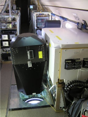
Atmospheric backscatter cross section as a function of altitude and time is shown in the top panel of Fig. 1. This data example was collected on September 6, 2010 during the Four Mile Canyon fire. Boundary layer aerosols extend to about 2 km at the start and end of the time period displayed. Above this layer the tropospheric backscatter cross section drops by one to two orders of magnitude. The smoke from the fire appears at 17 UTC and has backscatter cross sections one or two orders of magnitude stronger than those in the boundary layer. The bottom panel of Fig. 1 shows the depolarization ratio for the same time period. The smoke is much less depolarizing than those of the boundary layer and higher tropospheric aerosols. Extinction cross section is also simultaneously measured, although not shown in these plots. The smoke had an extinction cross section two orders of magnitude stronger than boundary layer aerosols.

Figure 1. GVHSRL measurements of aerosol and smoke at NCAR’s Foothills campus on September 6, 2010. Larger backscatter cross section and lower depolarization ratio delineate regions of smoke from ambient aerosols. Higher optical depth (> ~2.5) through the smoke limit the maximum range of the lidar to 4km.
Figure 2 is an example of airborne data. The calibrated backscatter cross section data in this figure is an example of a typical profile obtained during the Tropical Ocean tRoposphere Exchange of Reactive halogen species and Oxygenated VOC (TORERO) field project (note, the color bar scale is logarithmic with the number being the exponent). This atmospheric profile was performed off the coast of Chile on January 27, 2012. The GV aircraft is at an altitude of 7 km at the start of this time period, descends to 4 km for a short time, then continues to 100 m (at the bottom of the 1km deep marine boundary) then repeats the 4 km to 100 m profile. The lidar was switched between up (zenith) and down (nadir) pointing as the aircraft profiled the atmosphere. The lidar is useful in determining atmospheric layers of interest and guiding the aircraft into these layers for in situ measurements. Nadir or zenith pointing does not alter the retrieved backscatter cross section as FOV and gain differences between the four receivers are well characterized.
Figure 2. TORERO airborne backscatter cross section data example.
When particles orient, the scattering matrix has a different form than that of their randomly oriented counterparts. The scattering matrix has six degrees of freedom (backscatter, diattenuation, retardance and three independent depolarization terms) (Hayman and Thayer 2012) compared to the typical two (backscatter and depolarization) where scatterers are randomly oriented. By interrogating the entire scattering matrix, the HSRL is able to identify altitudes containing oriented ice crystals (Hayman et al 2012, Hayman et al 2014), Figure 3, and resolve all of the polarization terms, Figure 4. Because this measurement technique is relatively new (only previously performed by Kaul et al 2004), the exact benefits of these additional polarization terms are not well established. The additional information about the scattering volume may provide the means to better determine relative populations of oriented and randomly oriented particles, oriented particle size, habit and orientation distribution. Though these products are commonly applied to ice crystals, they have also been demonstrated with raindrops that flatten due to drag.
Figure 3. Time resolved profile from July 2, 2012 05:00 MDT of an ice cloud containing oriented ice crystals. The diattenuation profile shows the layer where the ice crystals are present.
Figure 4. The scattering matrix is decomposed into its five polarization effects. Disagreement between the three depolarization terms just above 5 km is an indicator of order in the system, suggesting the relative population of oriented ice crystals is relatively large.
Shupe (2007) describes a method for delineating regions of cloud liquid, ice and aerosol using backscatter and the depolarization ratio. It uses thresholds, or hard boundaries, to identify particle classes. The use of hard boundaries can lead to misclassification because there is a fair amount of overlap between observables for various particle types. Boundaries between most of the observables are “fuzzy” as there is a smooth transition from one article type to the next as demonstrated by Vivekanandan et al.(1999). In a fuzzy logic scheme membership functions are used to define boundaries between various particle types. Values of backscatter and depolarization ratio are passed to membership functions to determine the degree to which each observation belongs to a particular particle type. Hard boundaries between various particle types were “fuzzified” for classifying particles. Preliminary results based on the above described classification scheme are shown in Figure 5.
Figure 5. Vertical profiles of backscatter cross section, linear depolarization ratio and the corresponding particle classification. The lidar measurements were collected by the NCAR HSRL on July 18, 2010 at the University of Wisconsin.