Background
Prior to 2011, pressure transducers were installed in the housings of the NSF/NCAR GV dew-point sensors. The first projects for which these sensors were available were DC3-test and HIPPO-4. Prior to that time, for all GV projects up to and including PREDICT in 2010, these pressure measurements were not available and data were processed as if the pressure in the housings were the same as the ambient pressure. Once the sensors were installed, they indicated that the pressure in the housings was significantly different from ambient pressure, usually by being lower that ambient, an unexpected result.
Since 2011, projects have been processed with dew point measurements corrected for the measured pressure in the housing, as described in the document ProcessingAlgorithms.pdf, section 4.5. However, projects prior to 2011 have not been reprocessed to correct the dew-point measurements. This memo describes the basis for reprocessing. With the need to reprocess to correct temperature measurements, there may be an opportunity to include this dew-point correction as well.
Basis for Reprocessing
Although pressure measurements in the housings of the dew-point sensors were not available prior to 2011, since then we have had an opportunity to evaluate those measurements in many projects, including HIPPO-4/5, DC3-Test and DC3, TORERO, MPEX, SAANGRIA-Test, IDEAS-4-GV, SPRITES-II, and CONTRAST. To reprocess projects prior to 2011, we can use fits that predict the housing pressures on the basis of other flight characteristics, and we can use this large set of projects to assess if there is enough consistency in those fits to warrant applying them to old data. A preliminary look at this was discussed in this memo and this presentation, where a preliminary look at this approach was included along with discussion of how the pressure measurements are used and how significant they were. This memo now extends that analysis with data from additional projects.
CONTRAST
CONTRAST provides a good example. The measured ratios of the pressure in the housing of the two sensors to the ambient pressure are shown in Figs. 0.1 and 0.2. There is a clear change in the dependence of both pressure sensors at Mach 0.6, so separate linear fits were used above and below this Mach number. The best-fit coefficients are listed on the figures, and the fits were constrained to match at Mach number 0.6 to avoid discontinuous changes. The measurements and fits for the two housings are different, as expected because they are on opposite sides of the nose and so have different locations for the sensing holes relative to the fuselage and airflow.
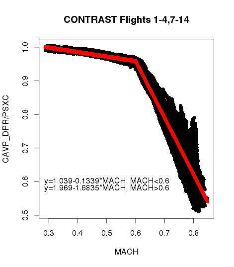
Figure 0.1:
The ratio of the pressure in the right dew-point housing to the ambient pressure for 12 flights from the CONTRAST experiment. The other five flights were omitted because the measurements were inconsistent with this pattern, sometimes because the instrument had malfunctioned and was undergoing service. Black dots are individual 1-s measurements, and the red line is the result of a linear fit to this ratio as a function of Mach number.
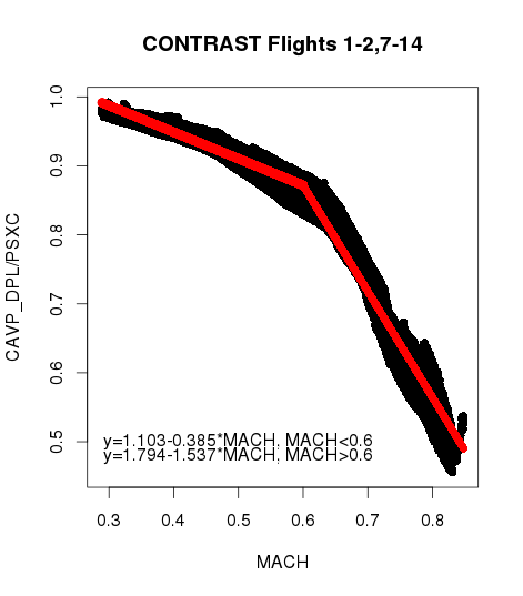
Figure 0.2:
As in Fig. 0.1 but for the left dew-point housing. Ten flights were used to construct this plot. Black dots are individual 1-s measurements, and the red line is the result of a linear fit to this ratio as a function of Mach number.
There are larger deviations from the best-fit line for DPR than for DPL, but they do not have much effect on the standard error of the fit. For DPR, the standard deviation of measured values about the fig shown in Fig. 0.1 is about 7 hPa and the standard error in the ratio of cavity to ambient pressure is about 3%. For DPL, the standard deviation of measured values about the fit shown in Fig. 0.2 is <6 hPa and the standard error in the ratio of cavity to ambient pressure is 2%. Because a 7% change in this ratio is required to produce a change in dewpoint of 1
C, a 2% or 3% standard error is tolerable relative to the expected uncertainty in the measurement. However, failure to correct for the 50% reduction in pressure present at Mach number above 0.8 would produce an error of around 10
C, which would be quite significant. This illustrates the importance of making these corrections to data from projects flown before the pressure measurements in the housing were available.
HIPPO-5
To check for universality of the fit obtained from CONTRAST, the fit procedure was repeated for the HIPPO-5 project, flown soon after the measurement of pressure in the housing became available. Flights 2 and 3 had some outlier measurements, possibly from encounters with ice crystals or icing, in the pressure measurements for the right housing, and flight 12 had similar problems for the left housing, so these were excluded. The pressure measurements (Figs. 0.3 and 0.4) appear very similar to those from CONTRAST, and the CONTRAST fits (shown as blue lines in those plots) are quite close to the fits determined from the HIPPO-5 measurements. Indeed, if the CONTRAST fits are used, the standard error in the measurements from HIPPO-5 are about 2% for both housings, so they are similar in error to that for the CONTRAST measurements and are also sufficiently low to introduce only a possible error of a fraction of a degree in dewpoint while correcting much larger errors that otherwise would be present.
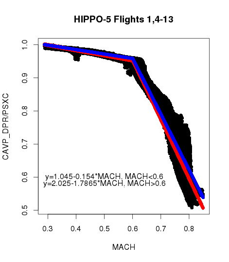
Figure 0.3:
As in Fig. 0.1 but for flights 1 and 4–13 of the HIPPO-5 project. The red line is the fit determined from these measurements (with coefficients as in the annotated lines), and the blue line is the corresponding fit determined from CONTRAST.
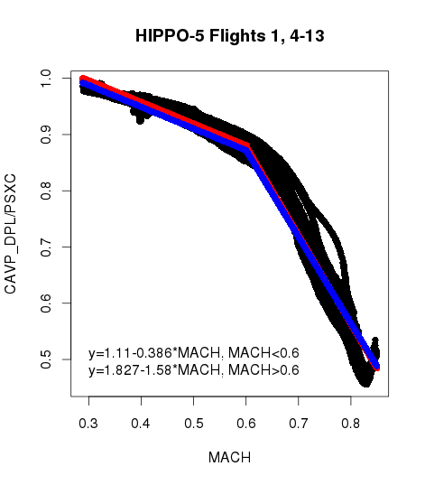
Figure 0.4:
As in Fig. 0.3 but for the left sensor and for HIPPO-5 flights 1, 4-11, and 13.
Recommendations
For projects prior to 2011 (PREDICT and earlier), calculate an expected housing pressure analogous to the measured pressures CAVP_DPR and CAVP_DPL and use them as in now-standard processing for the dewpoint measurements. They can be calculated from these equations:
For MACH < 0.6:
For MACH >0.6:
Processing can then follow the standard processing chain, but using these values in place of the measurements.
For the future, we should explore ways to avoid the large pressure drop in the housings because this is harmful to the response time and lower limit of the measurements.
Images