Calculation of soil heat flux at the surface

Calculation of Soil Heat Flux at the Surface

1. Ground Heat Flux (G)

The ground heat flux G is one of the components of the surface energy balance equation, describing the energy that is either taken up or released by the soil. We define the ground heat flux G to be positive when heat is conducted downward, away from the surface into the ground, and negative if heat is conducted upward toward the surface. The surface energy balance can thus be expressed as

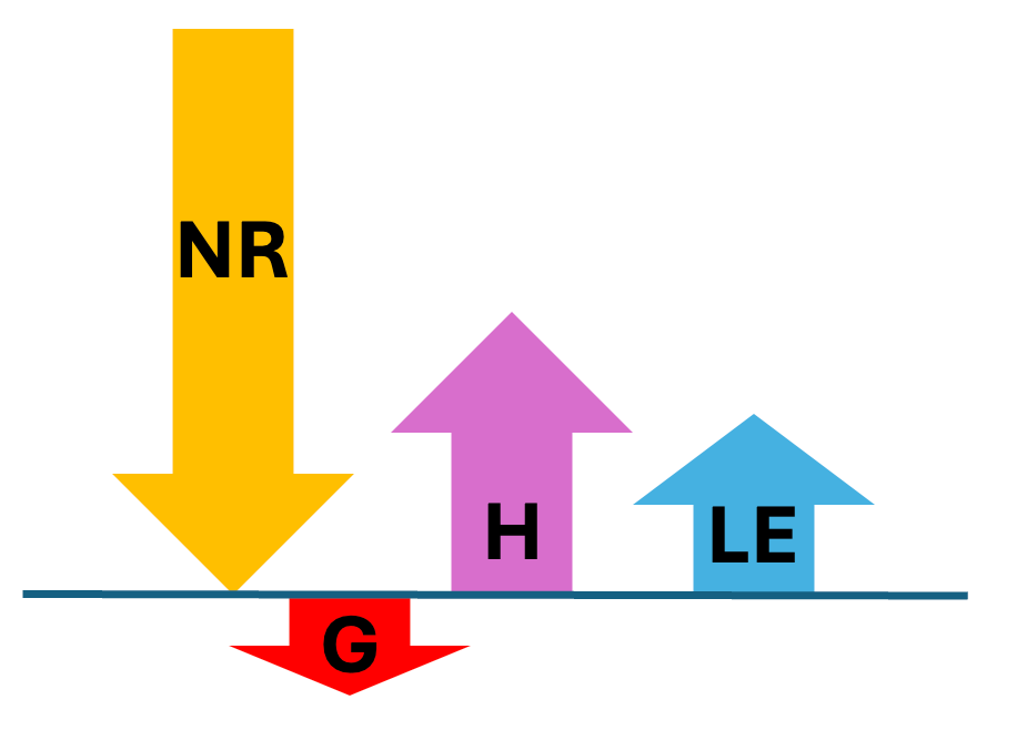
where NR is net radiation (positive towards surface), H and LE the turbulent sensible and latent heat fluxes (positive away from surface), and G the ground heat flux (positive away from surface).

Observations of G are made by combining measurements of the soil heat flux, Gsoil, at a certain depth (typically 5 cm) using a heat flux plate, with the flux associated with the heat storage change, Ssoil, of the soil column above that  plate. In the following we explain the measurement of these two components.

1.1 Soil heat flux at depth (Gsoil)

EOL/ISFS uses the REBS HFT3 sensors to measure the soil heat flux at a depth of 5 cm, Gsoil. These sensors have fixed dimensions and thermal conductivities, and are calibrated relative to a known heat flux through a water saturated glass bead medium of known thermal conductivity. We need to account for the effect of differences in the thermal conductivities of the heat flux plate and the medium in which the plate is embedded, both during calibration and our soil observations. Two Philips Corrections (Philips 1961) are used to account for both, the larger heat flux through the sensor during the calibration process, and the larger heat flux through the sensor during the measurements in the soil. The Philip correction f is expressed as the ratio of the heat flux measured through the heat flux plate G_p to the heat flux through the surrounding medium G_m, where G_m is G_c during calibration or G_s during soil observations. The correction is calculated based on the dimensions of the heat flux plate, and the thermal conductivities of the plate λ_p and medium λ_m. With a plate thickness of T and a plate diameter D,

The two Philips corrections are f_c and f_s, with the media either the water saturated glass beads during calibration or the soil during field observations, and f_c = G_p/G_c and f_s = G_p/G_s. The corrected heat flux through the soil, G_s, is calculated from the heat flux G_c based on the calibration coefficient by substituting for G_p, as: 

For the REBS HFT, the plate thickness T is 3.93 mm, the plate diameter D is 38.56 mm, and the thermal conductivity λ_p is 1.22 Wm⁻¹K⁻¹. The calibration medium of water saturated glass beads has a thermal conductivity λ_c of 0.906 Wm⁻¹K⁻¹ and thus f_c amounts to 1.053, and

f_s is determined using Equation 2 and the thermal conductivity of the soil, λ_s, measured by our Hukx (former Hukseflux) soil thermal property probe TP01. Note that the sign convention for Gsoil measurements with the REBS HFT3 is that a positive heat flux is directed downward through the heat flux plate.

1.2 Heat storage change above flux plate (Ssoil)

The second component of the ground heat flux, often referred to as the storage term Ssoil, accounts for the energy absorbed or released by the soil layer above the heat flux plate. It is calculated from the rate of change of the soil temperature and the thermal heat capacity of the soil layer. 

We measure soil temperatures (Tsoil) at the center of 4 soil layers, each 1.25 cm thick, covering the 5 cm above the heat flux plate. The Hukx (former Hukseflux) soil thermal property probe TP01 is used to determine the volumetric thermal heat capacity of the soil, C_v,s. We can thus calculate the individual storage terms for each of the 4 layers, and add it up to the total term:

                                                                                                                                                                (5)

Finally, the ground heat flux, G, is calculated as

References

Philip, J. R., 1961: The theory of heat flux meters. J. Geophys. Res., 66(2), 571–579, doi:10.1029/JZ066i002p00571.