AHATS
Advection Horizontal Array Turbulence Study
Advection Horizontal Array Turbulence Study
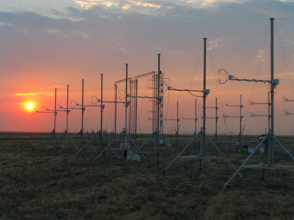
AHATS was a surface-layer turbulence study in the San Joaquin Valley, California, during the summer of 2008. The PIs on the project were Chenning Tong (Clemson), John Wyngaard (Penn State), Tom Horst (NCAR) and Peter Sullivan (NCAR). The NCAR facilities involved were the ISFS and the ISS. Data from these facilities can be accessed here.
AHATS was the fourth in the series of Horizontal Array Turbulence Studies (HATS). This series of experiments aims to improve large-eddy simulations (LES) of turbulence close to the Earth's surface, by collecting data that can be spatially filtered into scales that can be simulated by LES and those that must be parametrized.
The first was HATS, which was located in Kettlemen City, CA on fallow land with 19 anemometers. Then OHATS in Martha's Vineyard, MA on an over-ocean platform with 19 anemometers. The third project was CHATS which was done in Dixon, CA inside a walnut canopy with 30 anemometers. This project, AHATS is the most recent and was done in Kettlemen City, CA on fallow land with 33 anemometers.
HATS experiments:
| year | name | location | surface | # of anemometers |
| 2000 | HATS | Kettleman City, CA | fallow land | 19 |
| 2004 | OHATS | Martha's Vineyard, MA | over-ocean platform | 19 |
| 2007 | CHATS | Dixon, CA | inside a walnut orchard canopy | 30 |
| 2008 | AHATS | Kettleman City, CA | fallow land | 33 |
The first 3 experiments all used two horizontal lines of 9 sonic anemometers to provide cross-stream filtered velocity and temperature statistics. AHATS returned to the original HATS site, but a third line was added upwind to provide spatial differences in the streamwise direction. In addition, two horizontal lines of turbulent pressure sensors were added to AHATS to investigate, for the first time, resolved and parameterized pressure correlation terms in the turbulence transport equations. Those capabilities were unavailable in previous field programs but are important for understanding the SGS turbulence and for testing SGS models that are based on the SGS physics.
Chronology
| start (PDT) | end (PDT) | horizontal spacing | downwind heights | upwind heights | |
| June 9th, 2008 | setup begins | ||||
| June 25th, 12:00 | July 1st, 12:17 | widely-spaced array, lowest heights | 4.00 m | 3.24 and 4.24 m | 3.74 m |
| July 1st, 12:55 | July 18th, 05:55 | wide array, lowest heights | 4.00 m | 3.24 and 4.24 m | 3.24 m |
| July 20th, 16:00 | July 29th, 06:00 | medium-spaced array, lowest heights | 1.29 m | 3.64 and 4.64 m | 3.64 m |
| July 29th, 12:30 | Aug 8th, 06:00 | medium-spaced array, medium heights | 1.29 m | 4.83 and 5.83 m | 4.83 m |
| Aug 9th, 18:00 | Aug 16th, 09:00 | narrow-spaced array, highest heights | 0.43 m | 6.98 and 7.98 m | 6.98 m |
| August 16th | teardown begins |
Location
The site was on land owned by Westlake Farms in the central valley of California. According to the profile tower data system's GPS, the tower (which never moved) was at 36.02405 N, 119.90002 W. The ISS SODAR/RASS(?) was located about 270 m East of this tower and the ISS 915 MHz wind profiler/radiosonde system was set up approximately 5 km to the NW at 36.04968 N, 119.94202 W.
Sensor Data Post-Processing
Sonic Anemometer Data Editing
The AHATS sonic data have been edited to remove obviously bad data, putting NA's in the cal_files when the 5-minute averages of the sonic diagnostic variable exceeded ~0.5. During the first configuration, these usually occurred simultaneously on all channels of one of the four sonic adams, suggesting that the adam could not keep up with data ingest when there were transmission problems back to the base. After the first configuration, simultaneous problems on all channels of an adam occurred less frequently and with smaller 'diag' values. Then most of the high 'diag' values were associated with the beginning or end of a period of lost data.
For configuration 4, after August 8, sonic '6u' had recurring continuous periods in the middle of the day with 'diag' values between 0.05 and 0.1. I did not edit these out because it would have removed a significant fraction of the data from 6u during configuration 4.
Sonic Zero-Wind Offsets
Prior to the field project, all sonics were checked for zero-wind offsets at room temperature. Those with offsets larger than 4-5 cm/s were returned to the manufacturer for recalibration. Following the project, we repeated this test and found that 26 out of 41 sonics had offsets exceeding 4-6 cm/s. A few had offsets up to 20-30 cm/s. We do not know when or at what rate these changes occurred.
Subsequently, we have run each of the sonics used in AHATS in a zero-wind chamber inside a temperature-controlled chamber in the NCAR Sensor Calibration Laboratory to determine the offsets for each wind component. This is similar to one aspect of the manufacturer's recalibration process wherein offsets are determined as a function of temperature and entered into the sonic firmware for correction of the measured wind data. The chamber temperature was ramped from 60 C down to -30 C over a 6-hour time period (black lines), then back up to 60 C over a second 6-hour time period (red lines), and finally allowed to cool down with the temperature control turned off (green lines). Data collection was terminated at somewhat arbitrary times during the last cool-down phase.
The following table lists the sonics by serial number (and location) and includes links to plots of NCAR post-project measurements of the wind offsets as a function of temperature. The table also lists the maximum offset (cm/s) for each orthogonal wind component and the temperature at which the maximum occurs.
| CSAT S/N | Location*** | u.off | @T | v.off | @T | w.off | @T |
|---|---|---|---|---|---|---|---|
| Config 1, 2, 4 | cm/s | deg C | cm/s | deg C | cm/s | deg C | |
| CSAT-0247.pdf | 11t | 2 | 30 | 8 | 50 | -4 | 50 |
| CSAT-0364.pdf* | 8b | -6 | 20 | 8 | 20 | -7 | 35 |
| CSAT-0366.pdf | 10t | 7 | 35 | -6 | 40 | 4 | 50 |
| CSAT-0367.pdf* | 9t | 9 | 30 | 8 | 25 | 2 | 25 |
| CSAT-0369.pdf | 8m Aug 3rd - 5th 7m from Aug 5th |
-8 | 40 | -13 | 50 | -1 | 50 |
| CSAT-0370.pdf | 5t config 4 | 5 | 50 | -4 | 50 | -2 | 45 |
| CSAT-0376-offsets.pdf | 6b | 15 | 50 | -3 | 50 | 3 | 50 |
| CSAT-0377-offsets.pdf | 12b | 16 | 30 | -8 | 40 | -3 | 40 |
| CSAT-0378-offsets.pdf | 8t | 7 | 20 | 8 | 40 | -3 | 35 |
| 0536 | 4u | ||||||
| 0537 | 5.5m | ||||||
| 0538 | 10b | ||||||
| 0539 | 3u | ||||||
| 0540 | 7t | ||||||
| 0671 | 7b | ||||||
| CSAT-0672-offsets.pdf | 6t | 5 | 15 | 6 | 35 | -3 | 40 |
| CSAT-0673-offsets.pdf | 8u | -7 | 50 | 5 | 50 | 5 | 50 |
| 0674** | 6u | 20 | 25 | 12 | 30 | 1 | 10 |
| CSAT-0677-offsets.pdf | 5u | 5 | 20 | 12 | 30 | -5 | 50 |
| 0712 | 5t config 1-3 | ||||||
| 0720 | 7m until Aug 5th 8m from Aug 5th - 11th |
||||||
| CSAT-0732.pdf | 1.5m | -10 | 40 | 7 | 40 | 4 | 40 |
| 0733 | 8m until Aug 3rd 8m after Aug 11th |
||||||
| 0738 | 3t | ||||||
| 0739 | 3m after June 27th (also 13b config 2) |
||||||
| 0740 | 4m (13b config 3) | ||||||
| CSAT-0741.pdf* | 13b config1 2b config 2 - 4 |
15 | 50 | -30 | 50 | -3 | 50 |
| CSAT-0743.pdf* | 9b | -13 | 20 | 13 | 33 | 5 | 30 |
| CSAT-0744.pdf | 4b | -9 | 50 | -12 | 50 | -3 | 50 |
| CSAT-0745.pdf | 5b | 5 | 47 | 5 | 40 | -4 | 50 |
| 0800 | 3b | ||||||
| 0853 | 1b | ||||||
| 0855 | 11b | ||||||
| 0856** | 4t | 7 | 25 | 2 | 15 | -8 | 40 |
| 1117 | 2b config 1 | ||||||
| 1119 | 7u | ||||||
| CSAT-1120-offsets.pdf | 13b config 4 | 6 | 50 | 3 | 25 | -1 | 20 |
| 1121 | 9u | ||||||
| 1122 | 11u | ||||||
| 1123 | 10u | ||||||
| CSAT-1124-offsets.pdf | 3m until June 27th | -6 | 25 | 2 | 15 | 2 | 25 |
*cycle-slip errors cause jumps in temperature and wind offsets, generally at low temperatures
**data from Campbell recalibration
***Location notation: u = upwind (numbered from NE to SW); b = downwind, bottom; t = downwind, top; ht(m) = profile tower
Coordinate Rotation of Sonic Data
The data from each sonic have been rotated.
(a) about the sonic v (pitch) and u (roll) axes to correct for sonic tilt, where the rotation angles have been determined by the planar fit technique applied to each configuration period (or sub-configuration period when the sonic has been moved or replaced within the configuration period). To avoid flow distortion by adjacent sonics, the planar fit technique is only applied to data with wind directions within 45 degrees of normal to the array and wind speeds greater than 1 m/s. This technique assumes that the wind field, averaged over the configuration period, is confined to a plane parallel to the nominally horizontal underlying surface.
(b) about the sonic w axis to adjust for small differences in the sonic orientation relative to normal to the array, where the sonic orientations have been measured visually for each configuration using an optical Data Scope.
Sonic Wind Offset Corrections
The planar fit technique of step (a) above also derives an offset for the vertical velocity component of each sonic, which is subtracted from the sonic data, assuming that the mean velocity normal to the surface is zero.
Since post-project testing of the sonics found that many had offsets in the u and v wind components exceeding 4-6 cm/s, the sonic data has been corrected for offsets in the horizontal wind components as well. This was done by assuming that the time-averaged wind field was uniform across each sonic array. First the mean values of the horizontal wind components were calculated for each sonic over the period of each configuration, again for wind directions within 45 degrees of normal to the array and wind speeds exceeding 1 m/s. The wind offset corrections were then derived by selecting one or more reference sonics in each array with small post-project-measured offsets. These were sonic 8u (s/n 0673) in the upwind array, sonic 6t (0672) in the top array, and sonics 4b (0744), 5b (0745) and 6b (0376) in the bottom array. The u and v offsets for each sonic were calculated as the differences between its mean values for u and v and the mean values for the corresponding reference sonic. The offsets had a median value of 5 cm/s, but ranged up to a maximum of 33 cm/s.
Sonic Temperature Corrections
Small uncertainties in the sonic path length translate into non-negligible errors in the absolute temperature measured by the sonic anemometer. Campbell Scientific estimates that they can hold their path lengths to better than 0.3 mm out of 11.55 cm or about 0.26 percent. This gives a 0.26 percent error in the speed of sound, which in turn, gives a sonic temperature error of about 0.52 percent. At 300 Kelvin, this is a 1.6 Kelvin (or 1.6 deg C) error. In order to obtain uniform absolute temperature measurements across the horizontal arrays, we have made linear corrections to the sonic temperature for each sonic, assuming that the time-averaged temperatures are horizontally homogeneous. The coefficients are based on a linear fit for each configuration of the sonic temperature with respect to the speed-of-sound temperature calculated from temperature and humidity measurements on the nearby profile tower, interpolating the profile measurements to the height of the sonic. The offsets of the linear fits (in deg C) are on the order of 1 deg or less and the gains are within 2% or less of unity.
Sonic Heights
The sonic heights listed above were measured at the base of the booms (including 5.3 cm for the height of the sonic measurement volume above the top of the boom) on which they were mounted. Since these booms were not level, the sonic might actually be above or below that nominal height. The height difference was calculated from the sonic pitch angle that was determined from the planar fit technique,
height difference = boom - length * sin(pitch)
The mean height differences (cm) for each array and configuration period (or sub-period) are tabulated below. The Date/Time is the first time when the height difference applies. On July 1 the height of the upwind array was changed from 3.74m to 3.24m; and on July 31 the booms on the top and bottom horizontal arrays were lifted with guy wires to reduce their sag.
| date / time | upwind | top | bottom |
| June 25th, 12:00 | -0.1 | -0.3 | -0.4 |
| July 1st, 13:00 | -0.7 | -0.3 | -0.4 |
| July 20th, 16:00 | 2.1 | -3.0 | -5.6 |
| July 29th, 12:30 | 1.0 | -4.5 | -6.7 |
| July 31st, 17:00 | 1.0 | 3.2 | 0.9 |
| Aug 9th, 18:00 | 5.0 | 3.1 | 2.3 |
Pressure Sensors
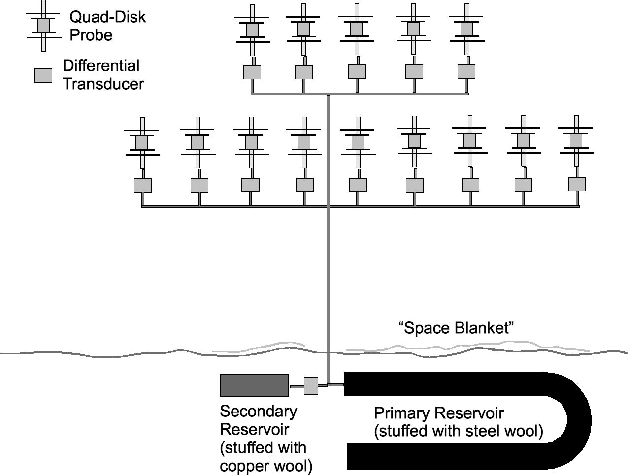
To attempt to measure the subgrid-scale filtered pressure field, 14 pressure ports, each with a high-frequency pressure transducer, were placed within the middle of both the top and bottom horizontal lines. The pressure ports were quad-disk probes of the design by Nishiyama and Bedard (NB) (1991) that were described by Oncley et al. (2009). Commercial versions of this probe were purchased from All Weather, Inc. (AWI), however wind tunnel testing of the AWI probes showed them to have larger errors than those made by NB. We modified the AWI probes by adding about ~7 cm of PVC pipe to the upper plate to make the entire probe more vertically symmetric, as suggested by Wyngaard (1988). This appeared to improve their response significantly.
Each port was connected through approximately 2 meters of 1/4 inch ID flexible tubing to the input side of a differential pressure transducer (Paroscientific Model 202BG). We expect little attenuation of pressure fluctuations below the Nyquist frequency of 5Hz from this tubing (Lenschow and Raupach, 1991). The 202BG is a digital sensor, with a frequency output for both the transducer temperature and pressure. These signals were ingested into two DSM boxes (pressure.1 and pressure.2) configured for this purpose with frequency counter boards. All of this worked as expected.
The reference side of all of the differential pressure transducers were connected together through thin tubing (1/16" ID?) to a reservoir that was buried in the ground and covered by a space blanket to maintain a relatively uniform temperature (and thus pressure, since the reservoir was sealed) [See diagram below]. During the experiment, leaks were identified and fixed in this tubing, the reservoir was enlarged (changed from an "empty" T-sized gas cylinder to a construction from 4" ABS pipe) and internal fluctutations were found in the reservoir and fixed (by stuffing the reservoir with steel wool). Even after all that, it was found that radiative heating + advective cooling of the reference tubing induced pressure fluctuations. Pipe insulation foam was added to cover this tubing, but it was still necessary to add a transducer to measure the reference pressure. Several different approaches to measure this pressure were used: a spare Vaisala sensor (first), a Paroscientific absolute pressure reference, and finally the NCAR pressure sensor that had been used in CHATS. Solving the reference pressure problems was the biggest challenge of the AHATS field crew.
AHATS Pressure System Diagram
Several modifications to the pressure system were done during the experiment to fix/test these problems. These are summarized (extracted from the logbook) below (times in PDT, UTC-7)
| date | note |
| Jul 6th, 15:30 | Get data from pressure1 |
| Jul 8th, 18:22 | Pref from Vaisala |
| Jul 9th, 10:00 | p.11b working (had been bad) |
| Jul 9th, 14:30 | Open tee leak fixed |
| Jul 10th | Leaks found in Tees |
| Jul 11th, 10:30 | Finished adding tiny cable ties to fix leaks (first good data) |
| Jul 13th, 15:20 | Improved output resolution of Pref |
| Jul 24th, 15:00 | Changed to CHATS reference |
| Jul 25th | Change to ABS reservoir |
| Jul 26th, 16:35 - 17:35 | Removed 11b for use as p.ref; added leak to ABS reservoir |
| Jul 27th, 10:11 | Pinched off leak |
| Jul 31st, 11:35 - 11:45 | Foamed part of reference tubing |
| Aug 1st, 08:00 - 08:40 | Foamed rest of reference tubing |
| Aug 2nd, 10:30 - 12:00 | P.0m (Paro) now best Pref; used p.11b on Bedard port |
| Aug 4th, 15:12 - 17:45 | Pinch tests on ref -- data bad |
| Aug 5th, 09:00 - 09:55 | Added stuffing to ABS reservoir; removed leak; p.ref reinstalled; P.0m to Bedard |
| Aug 5th, 14:40 - 15:22 | More pinch tests |
| Aug 6th, 10:33 - 11:34 | More tests; better seated ABS end caps |
Also after array switch of Aug 8, pressure2 was not running until Aug 9 19:50 GMT (12:50 PDT) and values for t.ref,p.ref (6, 3094, 3096) were zero until sometime after Aug 10, 16:00 (09:00 PDT).
Thus, the data have been processed using 5 cases:
- Don't add a Pref
- Use Vaisala Pref (should smooth, interp to 10 Hz) (Jul 8th to 26th)
- Use Paro P.0m (should smooth, interp to 10 Hz) (Aug 2nd to 5th)
- Use p.ref (Jul 26th to Aug 2nd; Aug 5th to end)
- Toss data (during leaks/tests/reconfigs/fixes)
There are some subtleties in how these reference values were added back in. Some amount of filtering and interpolating of the reference values was needed [more on this to be added].
Photographs
Plots
Data Access
- ISFS 5 minute average statistics in NetCDF format
- ISFS High-rate time series data available on request
- ISS (Integrated Sounding System) Data Page for AHATS
Links
Logbook
The AHATS logbook provides detailed information about the operation of the experiment. This page has other information as well.
Data Manager
EOL Archive, NCAR/EOL/DMS