
The following is from a paper written by Matt Beals.
The case studies presented are to demonstrate how the data archive can be used to study convective storms. The studies follow the previously outlined techniques and make use of the previously mentioned information concerning the instrumentation and storm structure. The studies make use of the archive data alone and in conjunction with outside data and analysis software.
Both case studies are of severe multicellular spring thunderstorms. The first storm is a strong, hail producing storm in which the aircraft has the opportunity to pass through cells in several stages of life as well as the remains of the storm after it dies out. The second storm studied is a weaker, yet still multicellular storm which presents a good opportunity to investigate some electrical properties of severe storms.
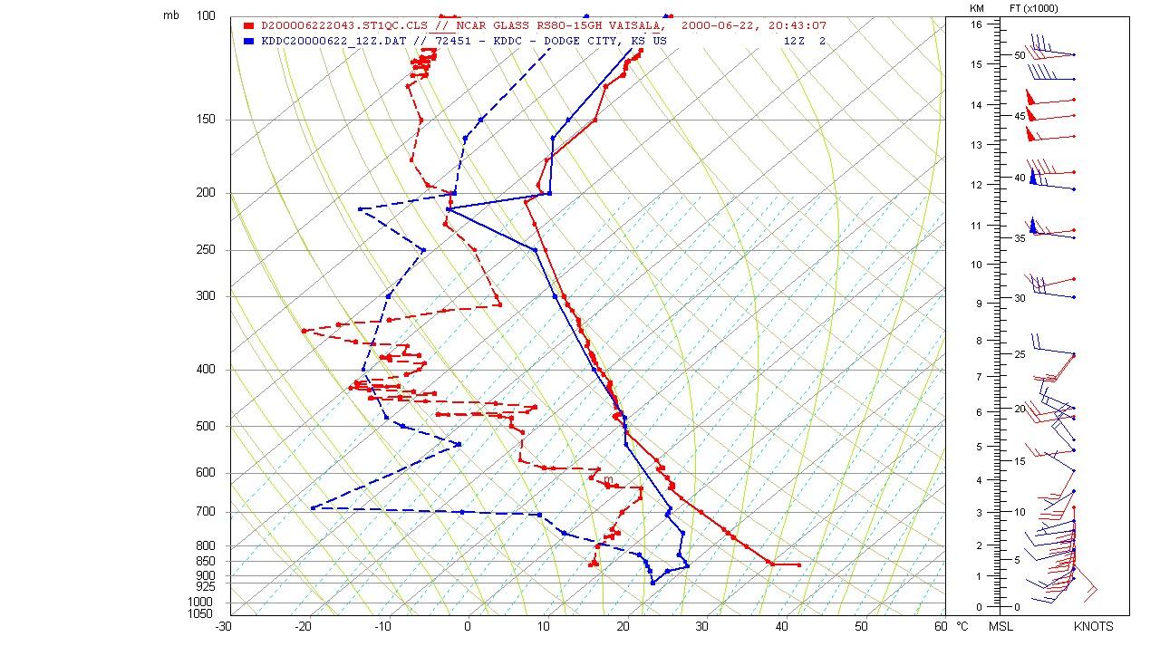 Figure 3.14 KDDC 12:00 UTC Sounding (blue) overlaid with MGLASS sounding taken at 20:42:07 (red)
The storm studied on June 22, 2000 occurred during participation in the Severe Thunderstorm Electrification and Precipitation Study (STEPS). The T-28 is based out of the Goodland, KS airport. Three radars are used during the project: the National Weather Service (NWS) WSR-88D located at Goodland (KGLD), the Colorado State University (CSU) CHILL radar near Burlington, CO and the National Center for Atmospheric Research (NCAR) S-Pol near Idalia, CO. The Goodland NWS office does not have the capacity to launch upper air soundings. This makes Denver (KDNR) and Dodge City, KS (KDDC) the two closest NWS daily upper air sites. During the STEPS project, MGLASS (Mobile GPS/Loran sounding system) units are used on an as-needed basis to provide on site soundings at a higher frequency. These soundings allow better analysis of the near-storm environment.
TopAn initial sounding is taken at the KDDC NWS office at 12:00 UTC on the 22nd, approximately eleven hours before the T-28 is deployed. RAOB is used to plot the sounding (Figure 3.14), which is retrieved from the NCDC archive. This sounding shows a strong inversion at the surface with moderate elevated CAPE. The hodograph shows some upper level speed shear, but is not supportive of severe thunderstorms. At 22:20:43 UTC, approximately an hour before the T-28 is deployed an MGLASS sounding is made nearby Goodland. The MGLASS sounding shows that the inversion noted in the KDDC sounding no longer exists. The wind shift between the two time periods, from south easterly to southerly, indicates that warm air advection at the surface caused the erosion of the inversion. Although the MGLASS sounding indicates a slightly weaker lapse rate, there is more moisture present in the mid levels. The hodograph also indicates that the environment is more supportive of strong thunderstorms, but does not suggest supercell type activity. The weak shear indicates that storms developing in this environment would be predominantly hail producers. It is also observed that the zero degree level is nearly coincident with the CCL, indicating that storms developing in this environment should contain a large amount of ice and super cooled water. This could possibly be problematic to the aircraft operations and instrument performance.
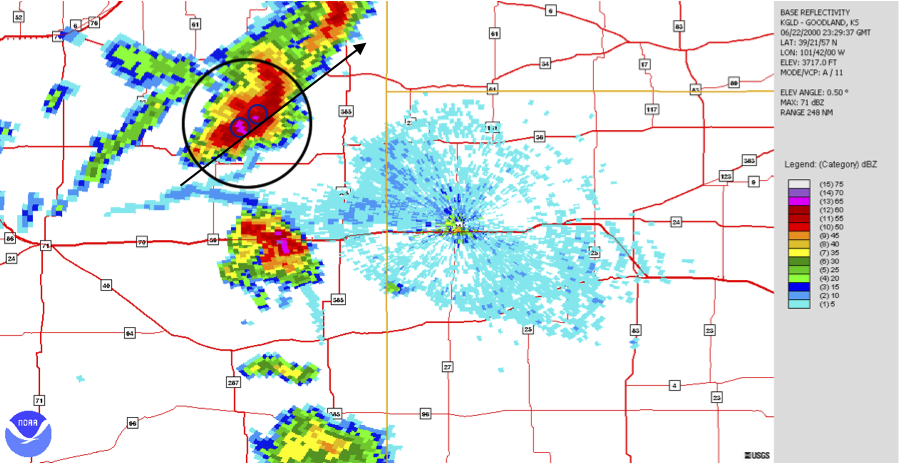
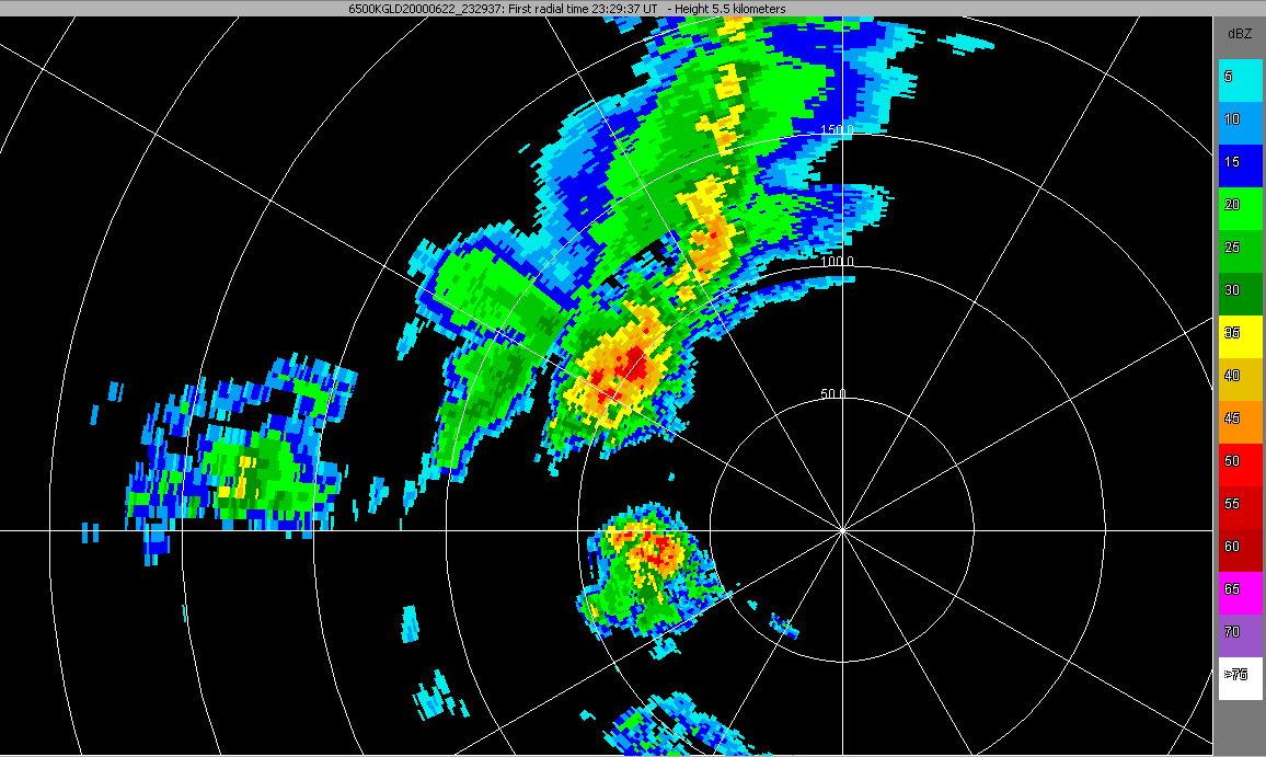 Figure 3.15: Radar summary for beginning of pass 1
According to the flight summary, the T-28 is launched around 5 PM MDT (23:00 UTC) from the Goodland airport. There are two storms tracking north-eastward to the west of the KGLD radar. A 0.5 degree base reflectivity scan plotted in java NEXRAD (Figure 3.15) shows both storms to have regions with reflectivity of 65dBz or greater. This is an early indication that both storms are producing hail. The northern storm (circled), which is chosen for the first pass with the T-28 shows a well developed outflow boundary extending to the south. This is an indication that the storm contains a well organized updraft and downdraft. There also appear to be regions of high reflectivity within the storm along the axis of storm motion. This is most likely evidence that the storm is multicellular and undergoing regeneration. Since the scan is a 0.5 degree scan, it represents the lowest portion of the storm. The larger size of the rear reflectivity core indicates that the hail is closer to the surface. This is typical in decaying cells where the updraft is no longer strong enough to support the elevated hail. The smaller region just ahead represents a stronger updraft that is still maintaining its hail aloft. Since the T-28 often flies higher then elevations sampled by the 0.5 degree scan, higher elevation scans are needed to see the environment sampled during the pass. The T-28 also attempts to maintain a constant altitude during a pass, so a Constant Altitude Plan Projection (CAPPI) is often useful in determining the storm environment sampled by the aircraft. The cross section of the flight track in Figure 3.16 shows that the aircraft maintained a fairly constant altitude for all passes within the storm. Reading the ordinate from the cross section reveals that the aircraft maintained approximately 5.5 km in altitude. The bottom radar image in Figure 3.15 is the 5.5 km CAPPI at the time of take off. The radar scan shows distinct reflectivity cores, reinforcing the multicellular nature observed in the 0.5 degree scan. The field report from the project, on the flight information page, indicates that the storms are forming off the southern end of a well organized MCS. Analysis of a radar loop generated with java NEXRAD (not shown) indicates that during the duration of the flight, the southern storm in the image tracks to the north and collides with the northern storm around 00:00 UTC. This complex then tracked to the east-northeast. According to the STEPS project report, the storm produced one inch hail, 30 m/s surface winds and a brief, weak tornado.
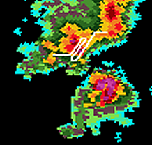 Figure 3.17 Radar image at 23:58 UTC with overlay of T-28 Flight track. The pilot entered the storm from the west, putting him at the south east side at the time of the image. The track indicates two passages through the primary regions of high reflectivity.
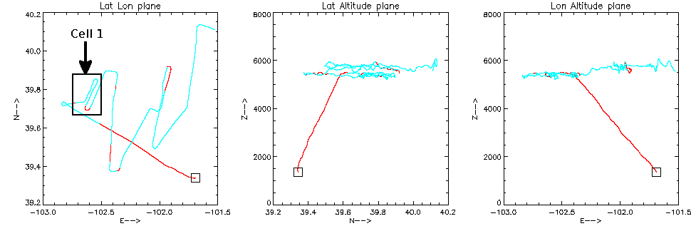
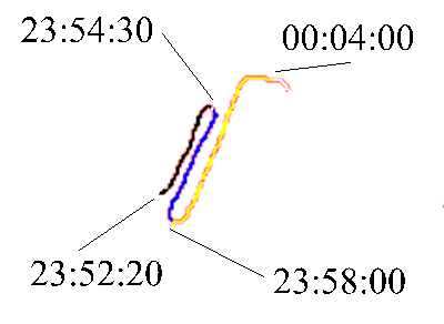
The T-28 took off from Goodland airport at 23:29 to intercept the northern storm. The aircraft continued to focus on that particular storm until the collision at approximately 00:00 UTC, at which time the aircraft began interrogating the newly formed complex, making passes further to the south. The T-28 followed the storm as it tracked eastward, focusing on the central reflectivity core. For the duration of the flight, the aircraft maintained between 5000 and 6000 meters in altitude. Figure 3.16 shows a flight track plot from the T-ADP. The penetration of the first storm, which is the focus of this discussion, is broken into three passes. The first pass starts at 23:52:20 and lasts until 23:54:30, the second pass starts at 23:54:30 and runs to 23:58:00 and the final pass begins at 23:58:00 and runs until 00:04:00. The first two passes are through the main developing cell while the third pass is the aircraft passing though the remnants of the storm after it begins to decay. Figure 3.17 illustrates his progress through the storm for each of the passes. These passes are determined by first identifying the portion of the track in which the aircraft is penetrating the storm in question. The plan view of the flight track (far left image of Figure 3.16) indicates three main passes through the storm, neglecting the portion of the flight in which the aircraft is climbing to penetration altitude. The beginning and ending times of these passes are determined by adjusting the time range in the T-ADP until the desired section of the flight track is highlighted.
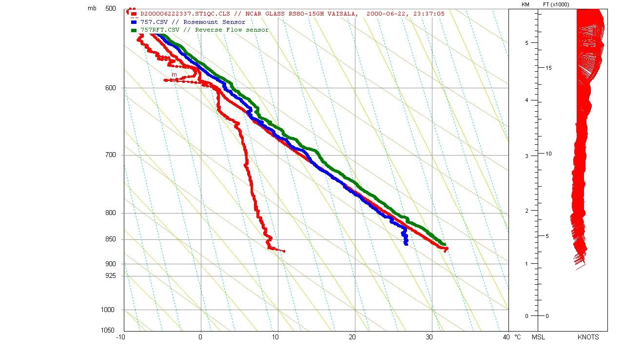 Figure 3.18 MGLASS sounding overlaid with recorded temperature data from the T-28 during ascent.
As the T-28 gained altitude setting up for the first pass, the instruments are recording pressure and temperature data. Using this data, an aircraft based sounding can be reconstructed to gain insight into the temperature structure of the atmosphere in the storm environment. This is accomplished by downloading the netCDF data file for the flight and reading the time, temperature and pressure data into IDL. By adjusting the time range on the T-ADP, the time of the end of the ascent is found. This time is then used in IDL to find the range of temperature and pressure values for the ascent period. These pressure and temperature values are printed to a text file, which is then formatted to be read by the RAOB program using the template included with the RAOB software. Since a standard sounding only contains one temperature record, one file for each temperature instrument is created. These files can then be opened in RAOB to generate the soundings seen in Figure 3.18. To gauge the accuracy of this method and the accuracy of the instruments onboard the T-28, this sounding can be compared to one taken by a MGLASS radiosonde launched minutes before take off (Figure 3.18). Overlaying all three soundings in RAOB shows that in general, the temperature profile recorded by the T-28 is very similar to that recorded by a radiosonde. This implies that such a sounding could be very useful in projects which did not make use of special soundings, or did not have a launch near the time or location that the T-28 began operating. However, the Figure does bring up some issues with the temperature data that need to be addressed. The first thing to notice about the plot is that there is moisture data only for the MGLASS sounding. This is due to the lack of a humidity measuring instrument onboard the T-28. Two primary trends in the behavior of the instruments are also observed. At the beginning of the record, the Rosemount unit (blue line) reads a brief isothermal layer that the RFT unit does not. Since the Rosemount is much more prone to wetting and following the wet bulb profile, this layer could indicate that the sensor is wet and read cold until it either dried out on its own or the pilot engaged the deicing circuits. Once the Rosemount unit starts following the actual atmospheric profile, there still is a discrepancy between it and the RFT's reported temperature. This difference is greatest at low altitudes and decreases as the pilot approaches the top of this climb. This discrepancy is most likely due to sensitivity of the RFT unit to rapid changes in temperature and aggressive angles of attack. Given that the aircraft is rapidly gaining altitude while recording this data, it follows that the atmospheric temperature is falling quickly and that the pilot is holding high angles of attack, which leads to a certain amount of error. As the pilot nears the target altitude and begins to slow his climb and decrease the angle of attack, the temperature profiles converge, indicating that the error is related to the climb.
TopTo begin analysis of the data recorded during the penetration, a general survey of several variables is completed to isolate regions of interest and regions which possibly could be contaminated with data artifacts. This general overview consists of four variables plotted in T-ADP: FSSP liquid water, 2DC particle counts, updraft speed, and temperature difference. The liquid water content of the storm plays a large role not only in products that involve liquid water but in the performance of the other instruments. The majority of contaminated data comes from probes icing over or from liquid water collecting on probe's structure and then bleeding off in front of the optics. The 2DC particle count plot indicates where in the cloud there exists slightly larger particles than what the FSSP is sensitive to. This can be an indicator of ice and graupel. The updraft plot provides a quick way to visualize the dynamics of the storm. Given that updrafts generally contain higher concentrations of liquid water and downdrafts contain lower concentrations, cross comparison between the liquid water plots and the updraft plot serve to help identify potentially problematic regions in the data. The temperature difference plot indicates when the two temperature sensors are reading differently, which would lead to errors in other calculations that rely on temperature data. Knowing that the Rosemount unit tends to read cold in regions of high liquid water, this variable can serve as another indicator as to when water fouling is occurring.
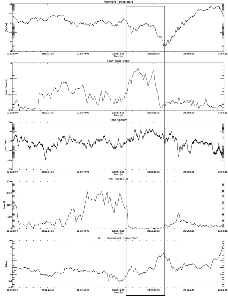 Figure 3.19. FSSP LWC, DMT LWC, Updraft speed, and Temperature difference.
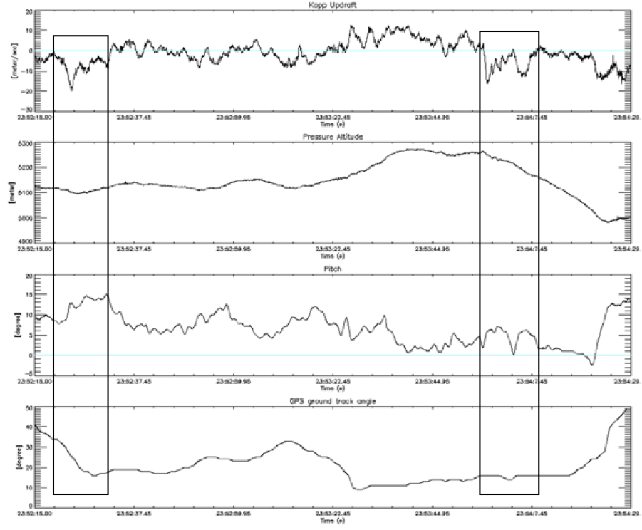 Figure 3.20 updraft, hail concentration, pressure altitude, pitch, and ground track angle.
The DMT probe is broken before take off and is registering negative liquid water values. This means that there is no direct means of verifying the FSSP liquid water data, so independent measures of liquid water content will have to be inferred from other instruments. The FSSP plot in Figure 3.19 indicates one region of significantly elevated liquid water. Comparison to the updraft plot indicates that this peak corresponds to a region of vertical motion. This region is indicated with in Figure 3.19. It is interesting to note that in general, the FSSP liquid water concentrations noticeably drop after the initial peak. This drop is somewhat related to the edge of the updraft, indicating that it could be a real drop in liquid water but it could also indicate the presence of ice buildup on the FSSP's optics and will require further investigation. The temperature plot indicates temperatures -4° C and colder. These temperatures indicate that all liquid water present is in a super cooled state. The temperature difference plot shows a large increase after encountering the first updraft and peak in liquid water. Since the temperature difference is computed by subtracting the Rosemount temperature from the RFT temperature, this indicates the Rosemount unit is reading cold. This is most likely due to the unit ingesting water, which is logical as the aircraft is passing through a region with elevated liquid water. It also indicates that there might be more liquid water present after that point than what the FSSP is reporting and is further evidence that the FSSP, and other optical probes, are becoming iced over. The FSSP liquid water trace indicates that the liquid water falls off just prior to the edge of the updraft, but the temperature difference indicates that there is still enough liquid water to wet the Rosemount unit well past that point. After the edge of the recorded updraft, the temperature difference drops dramatically, indicating the aircraft has moved past the region of high liquid water. The fact that the FSSP signal dropped out rapidly and that there is evidence of elevated liquid water where the FSSP is reading low concentrations is evidence that the probe could be icing over. The 2DC shadow/or variable, which can be equated to ice particle concentration, also shows a dramatic drop during the indicated time of updraft. Updrafts are typically dominated by liquid water and very little ice and this is consistent with the observed drop in 2DC concentration.
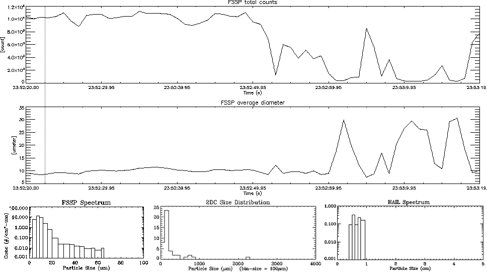 Figure 3.21 Detail of pre-updraft environment
Figure 3.19 also indicates regions of downdraft. Figure 3.20 is a T-ADP plot illustrating updraft strength, and some aircraft flight variables used for diagnostic purposes. In this Figure, downdrafts observed in the updraft trace are highlighted. When identifying downdrafts, it is a good practice to include a plot of at least the GPS track angle. Identifying the regions in which the aircraft is turning gives a good indication where artificial downdrafts will be observed. The first downdraft highlighted in the Figure appears to be very strong, in but comparison to the pitch and GPS track angle reveal that it is an artifact generated by a turn. The second downdraft highlighted is an actual downdraft. It is accompanied by no change in GPS track angle, lower values of pitch and a drop in altitude.
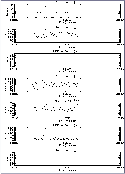 Figure 3.22 Particle Habit classifications pre-updraft environment
Figure 3.21 illustrates the recorded FSSP average diameter trace with the FSSP total counts variable for reference generated in T-ADP for the first half of the pass, ending just before the main updraft is encountered. Also included are histograms of particle sizes taken by the FSSP, 2DC and Hail spec at the beginning of the time period generated in T-28 display. The blue vertical dashed line indicates where in the time series the histograms are taken. Zooming in on the data in this fashion allows for a smaller region to be studied in higher detail. By excluding the region of updraft, the axis scales are enlarged to show greater detail. The FSSP spectrum shows a distribution weighted towards the small end with a mean diameter of 10 μm. This is the same information portrayed in the plot. The 2DC and hail distributions also show dominance toward smaller particles and at lower concentrations. This region of the storm appears to be dominated by liquid water and small ice. The apparent jump in average particle diameter towards the end of the trace is an artifact created by a low number of samples. Image classification using T-28 display of the particle images taken by the 2DC probe during this time period reveal in Figure 3.22 that approximately half of the hydrometeors sampled are tiny, uncategorizeable particles. These particles could be either small cloud drops or small ice particles. Since the FSSP tends to record small ice as larger particles, and the FSSP size distribution shows a heavy bias towards smaller particles, this region of cloud is most likely to contain mostly liquid water. Also present in slightly smaller concentration are nearly circular, regular and irregular particles. The nearly circular particles are a strong indication of rain drops, while regular and irregular particles are usually ice and graupel. This combination of small ice and rain on the rear flank of the updraft matches the model suggested by Krauss and Marwitz (1984).
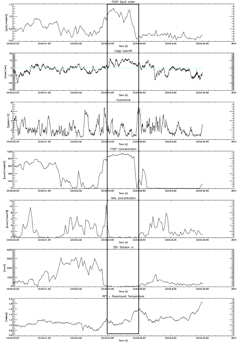 Figure 3.23 Particle concentration data with updraft and turbulence
The next region of the pass examined in detail contains the main updraft. According to the conceptual model, an updraft contains elevated liquid water, strong vertical motion and little ice. The region surrounding the updraft also is marked by increased turbulence. This makes, updraft, turbulence and hydrometeor related plots of particular interest. Since the Rosemount unit is prone to wetting in high liquid water environments, watching for a drop in Rosemount temperature compared to RFT temperature can be a good verification that liquid water is present. This is especially important in this flight, where the only source of liquid water information is from an imaging probe prone to ice error. Figure 3.23 shows a T-ADP plot of the previously mentioned variables. There appear to be two fairly small but strong updrafts prior to the main updraft, which is much larger in diameter. The edges of the updraft are marked by regions of downdraft, low liquid water concentrations and increases in hail concentration. The hail concentration and 2DC Shadow/or traces indicate that there is a higher concentration of hail and ice on the rear side of the updraft. This is consistent with the Krauss and Marwitz (1984) model. The edges of the updraft are also marked by higher turbulence than the interior sections. The turbulence plot indicates two main spikes in turbulence, which define the main edges of the updraft. There are smaller peaks in turbulence within this region that also coincide with smaller peaks in updraft strength. The elevated liquid water, decrease in hail and large ice, and presence of updraft-edge downdrafts all indicate that the larger region is defined as the updraft core. Because there is still intermittent turbulence in the updraft core, there is the possibility that the pilot is not flying through the middle of the updraft core and is experiencing turbulent mixing occurring along the edge.
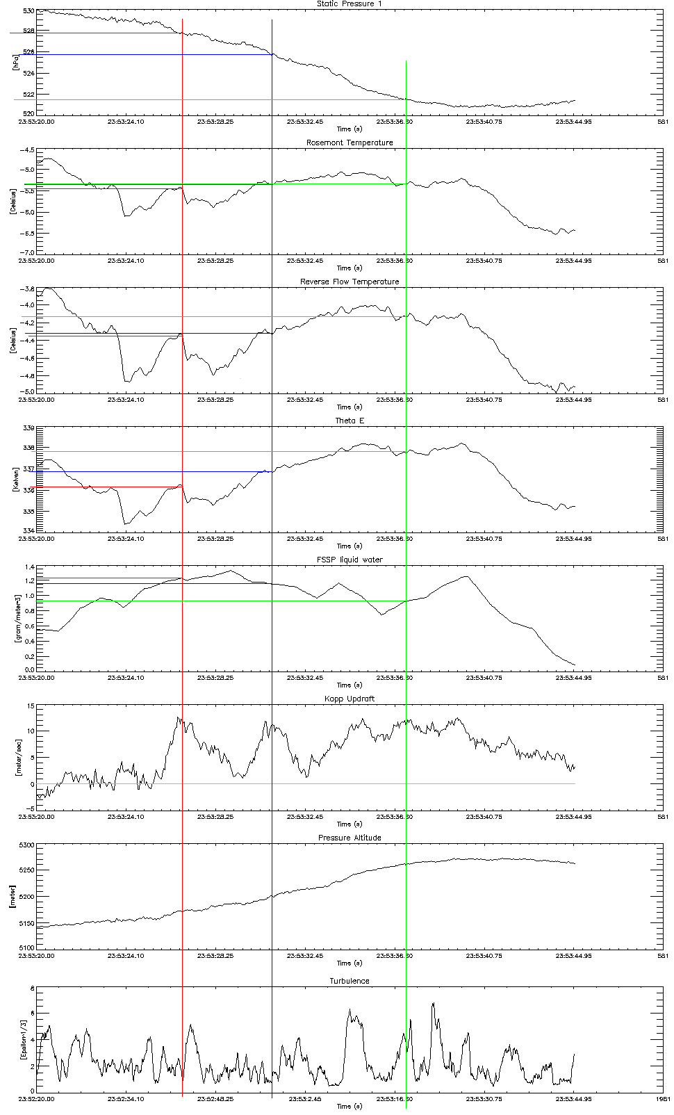 Figure 3.24 Thermodynamic properties of the first pass through the updraft
The center of the updraft contains elevated levels of liquid water and very little ice. The lack of ice in the updraft core indicates that, unless dry air entrainment is occurring, the updraft core should be close to adiabatic. Figure 3.24 shows a detailed section of the updraft, looking at temperature, pressure, equivalent potential temperature, LWC, updraft, and turbulence. This plot is generated in T-ADP and then modified in a standard image editing program. This allows for straight lines to be drawn across the plots, helping to correlate features and read values from the axis. Three peaks in updraft are identified and marked with red, blue and green lines. The first updraft, highlighted in red, corresponds to a rather abrupt increase in temperature and is bounded by two regions of higher turbulence. The second updraft, highlighted in blue, is again bounded by two spikes in turbulence, although they are not as clearly defined. There is a corresponding increase in temperature, but it does not drop like observed in the first updraft. The third updraft, represented by the green line, is the main updraft. Its width is on the order of 4 times the width of the previous updrafts. The updraft plot shows a long sustained region of updraft, but the turbulence data does not suggest the near laminar flow typically experienced. This is most likely due to the pilot flying very close to the edge of the updraft instead of in the middle of it. This observation supports the previous hypothesis that the pilot is flying on the edge of the updraft and experiencing the entrainment region, rich with turbulent mixing.
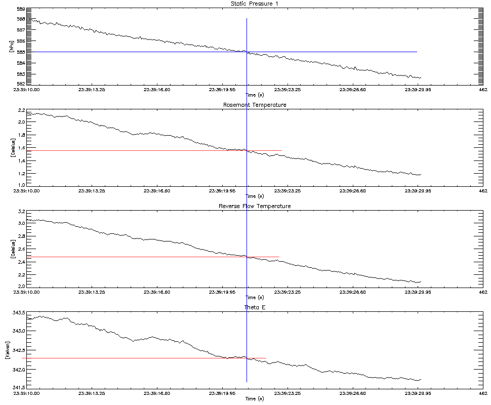 Figure 3.25 Cloud base measurements of temperature and equivalent potential temperature
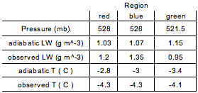 Table 3.2 Observed LWC and temperatures and adiabatic LWC and temperatures for three observed regions of updraft.
Another more detailed analysis of the data involves exploring the thermodynamic properties of the updraft. This is performed by both calculating the theoretical adiabatic temperature and liquid water contents at the penetration altitude and by comparing observed values of equivalent potential temperature in the updraft to those taken at the cloud base. This should give an indication to the amount of entrainment in the updraft. The values of 275.05 K and 585 mb for the cloud base temperature and pressure respectively are obtained during the initial take off of the aircraft. The cloud base altitude is estimated from the CCL on the sounding and the lowest pressure level at which the pilot reported cloud. In some cases, the pilot will estimate the cloud base altitude which is recorded in the flight video or the pilot log. A plot from T-ADP of the thermodynamic properties observed during take off is marked with the estimated cloud base (Figure 3.25). Values for the adiabatic temperature and LWC are calculated for the three observed updrafts and displayed in table 3.2. Figure 3.24 displays the traces of temperature, liquid water and others used for the analysis. The first two updrafts observed both contain higher than adiabatic liquid water contents, but colder than adiabatic temperatures. The flight video during this time period revealed the pilot reporting hail. This indicates that ice is present in the initial two updrafts and that the liquid water content reported by the FSSP could be higher than actual. This implies that it could be much closer to adiabatic than indicated. The temperature used in the comparison is from the RFT probe, which is known to have systematic bias. Review of the sensors' performance throughout the flight indicates that even in clear air, where the RFT should agree with the Rosemount, the RFT is still reading approximately one degree colder. Factoring in the 0.5 degree precision of the probe, this puts the adiabatic temperature within the range of the observed temperature. The temperature comparison for the third updraft follows the same pattern. The video during the time of the third updraft shows a noticeable drop in the number of particles impacting the camera lens. This indicates that the ice present in the previous updrafts is not present in the third one. The observed lower liquid water could be a more realistic measurement due to less ice contamination. Combining the lower than adiabatic liquid water with temperatures which read colder than adiabatic (but could be close when error is considered) shows that the region of the updraft sampled is most likely less then adiabatic.
To further test the updraft for signs of entrainment, cloud base measurements of equivalent potential temperature are compared to those taken inside the updraft. In the free atmosphere, Theta E monotonically decreases with height and then begins to increase again near the tropopause. Since Theta E is conserved in adiabatic processes, an updraft, which advects air from lower levels to higher levels, would display higher Theta E values then the surrounding air. Since Theta E is conserved, the Theta E value of the air in the updraft should be the same as the source of the air, which implies that for a mature updraft, it should match the Theta E of the air at the cloud base. Theta E is calculated from the recorded temperature, assuming that the air the aircraft is sampling is saturated. Theta E is calculated for both the Rosemount and RFT probes, but only the value based off the RFT probe is used for this analysis. This is due to the tendency of the Rosemount probe to read cold in environments containing high quantities of liquid water. Since the Theta E values are of importance in updrafts, where liquid water is high, the RFT probe is a better option. The RFT is known to have a bias compared to the Rosemount, but since all calculations are being based off the RFT probe, this error is mitigated for the purpose of comparison. The initial updraft shows the lowest θe with a value of 336 K. The cloud base value is 342 K. Compared to the surrounding environment, the θe and temperature values are elevated, indicating that the updraft air is being advected from below. The second and third updrafts do not have individual peaks in temperature or θe but rather happen during a longer gradual increase in the values. This indicates that the last two updrafts are most likely fluctuations of the same updraft. Values of θe for these two peaks increase to 337 K and 338 K respectively, but do not approach the cloud base value of 342 K. This indicates that some mechanism is either cooling the air within the updraft or removing moisture from within it. This could be caused by several mechanisms, including dry air entrainment, or precipitation fallout.
The separation between the three updrafts is not an actual downdraft, but a region of lesser updraft. This indicates that the updrafts are cells or regions of elevated updraft which would be consistent with regions of turbulent mixing in the updraft wall. Measurements of θe indicate that the region of the updraft sampled is not adiabatic, which is reinforced with the observations made comparing the observed temperature and liquid water to the respective adiabatic values. However, the liquid water and temperature observations do indicate that small regions could be close to adiabatic. The turbulence profile also does not suggest that the pilot flew through a solid updraft, but rather through a region of updraft containing smaller scale vertical motions conductive to mixing. The observed particle data does suggest that the updraft interrogated is the central updraft of the storm, but remaining data confirms the original hypothesis that the main section of the updraft is not sampled, but rather the edge of it.
TopAfter exiting the updraft in the previous section, the pilot turns the aircraft around and reenters the storm on a reverse heading. Recalling from the previous pass, and the conceptual model of storm structure, the pilot will encounter a region of ice and growing hail in front of the main updraft and a region of larger hail behind it. The main updraft should be characterized by high liquid water with little ice and be bounded by spikes in turbulence.
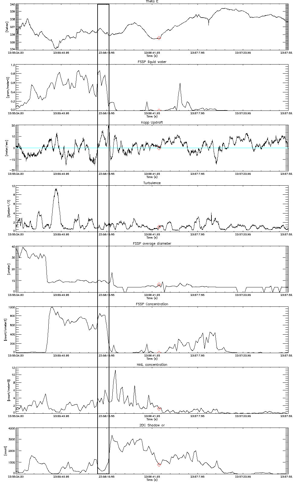 Figure 3.26 Observations for second pass.
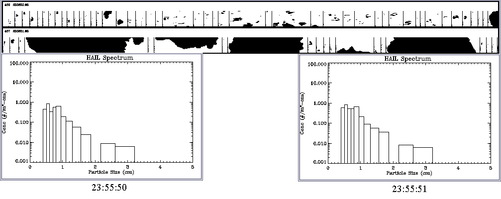 Figure 3.27 Hail size distribution and sample buffers from 23:55:50 to 23:55:51.
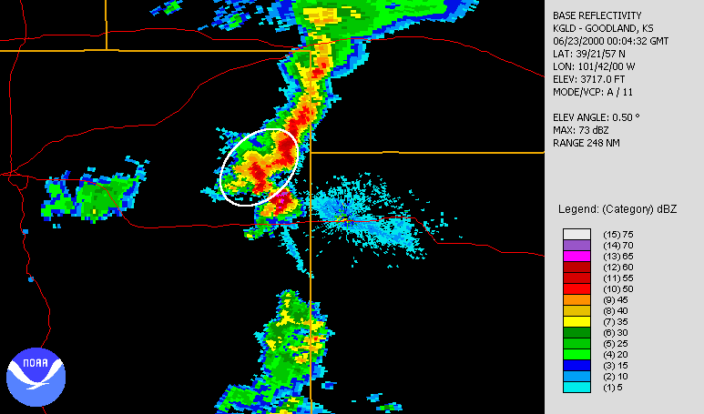 Figure 3.28 00:04:32 base reflectivity.
The main updraft core is identified in a T-ADP plot of updraft, turbulence, theta e and hydrometeor variables (Figure 3.26). As the pilot approaches it from the north, he passes though a region of elevated liquid water, ice and hail, indicated by peaks in the liquid water content, 2DC and Hail plots. This is the region of hail growth, with pockets of up and downdraft, where ice ejected forward of the updraft is being recycled back into the flow. Ice is evident in this region from the 2DC and hail trace as well as the flight video in which larger particles can be seen impacting the lens. The ice also manifests itself in the FSSP liquid water data. The beginning of the plotted time period contains a region with reported liquid water, but a very low concentration of particles. During this time, the FSSP probe is reporting that the mean particle size is 30 μm in diameter. This is a strong indicator that the FSSP is sampling mostly ice particles at the time. This period also contains some updrafts and downdrafts. The region of growth out ahead of the storm (to the north in this instance) is typically characterized by general updrafts. The region of downdraft experienced is consistent with the hypothesis that the storm is multicellular in nature, as the cells in the decay phase, which would be dominated by a precipitation downdraft, would be located out ahead of a strong downdraft. Size distributions from this downdraft indicate the presence of hail up to 32 mm (Figure 3.27). This indicates that the downdraft encountered is a remnant precipitation downdraft from the previous cell currently in the decay phase.
Immediately after encountering the decaying cells out ahead of the main cell, the pilot enters a strong updraft-edge downdraft prior to entering the main updraft. This downdraft is not correlated with any noticeable increase in particle concentration and is clearly an updraft-edge downdraft. There is another downdraft with similar strength and characteristics on the rear (south) side of the updraft. Strangely, the updraft does not show the expected increase in liquid water. There is a local peak, but it is not elevated in relation to the prior environment. Theta E values observed in the peak of the updraft are around 336 K, which is consistent with the previous pass through the updraft. The remainder of the penetration is dominated by variable up and downdrafts with gradually decreasing 2dc activity. This is indicative of the aircraft passing though the forming updrafts and downdrafts of new cells, as well as cloud edge downdrafts.
Top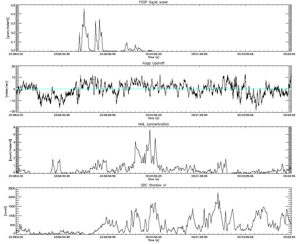 Figure 3.29 Updraft and hydrometeor data for the third pass
A 0.5 degree radar scan from java NEXRAD (Figure 3.28) indicates that by the end of pass three, the storm greatly dissipates. Reflectivity in the core is now topping out at 60 dBz. This indicates that precipitation is falling out of the storm; the cell is decaying and another strong updraft is not developing. In this scenario, the storm structure begins to decline. Since the updraft can no longer support the growing ice in the upper levels, it begins to fall out. There will still be pockets of updraft present, but they will be less organized. There should be an observed increase in the concentrations of mid-sized ice, as the growing hail embryos fall into the mid levels of the storm. The region previously occupied by the updraft and the downdraft should now contain large hail.
Analysis of the video reveals that the initial part of the penetration is largely in a cloud free environment. In fact, the pilot reports reentering cloud at 23:59:09, more then a minute after the beginning of the time period. Throughout the penetration the pilot reports encountering high turbulence and a few small updrafts, but no distinctive features manifest. This is apparent in the T-ADP plot of liquid water and hydrometeor variables as well (Figure 3.29). There are two distinctive downdrafts recorded, but these are during the times the pilot is turning to start the run and turning to exit, thus they are artifacts.
In the center of the pass, which is the region corresponding to prior location of the main updraft and downdraft, there are elevated hail concentrations. This is the elevated hail falling out of the storm. The updraft plot in this region shows that the strong updraft prevalent in the previous two passes has significantly weakened. After this peak in hail, the large hail recorded by the HAIL decreases, but the mid size ice recorded by the 2DC remains elevated, indicating the fallout of the growing hail embryos and graupel. During this period, the ground crew informs the pilot that the storm is dead and that he needs to set up to approach the storm to the south.
TopThis storm presents an opportunity to analyze a strong hail storm and explore the intricacies of multicellular structure. The general approach taken in the analysis is to attempt to determine what features should be visible in the data record by analysis of the radar plots generated in java NEXRAD and the large scale plots generated by T-ADP. An initial overview of the flight track in T-ADP serves as a good tool to divide the flight into several passes, but the external radar data is really required to fine tune the analysis and determine exactly which regions of the track are important to analyze. The radar data also helped a great deal to steer the analysis in terms of what features to expect. This is greatly enhanced by the ability to manipulate the data in IDL and generate custom analyses and plots.
The T-ADP greatly aided in this analysis. This presentation of the data shows the final product of the analysis. It does no show all of the manipulation and comparison of different plots performed until a final, polished product is generated. This manipulation and comparison is what takes the majority of the analysis time. The T-ADP allows for quick, easy and precise manipulation of the time scale and the variables plotted, making this exploration process very quick and efficient.
Top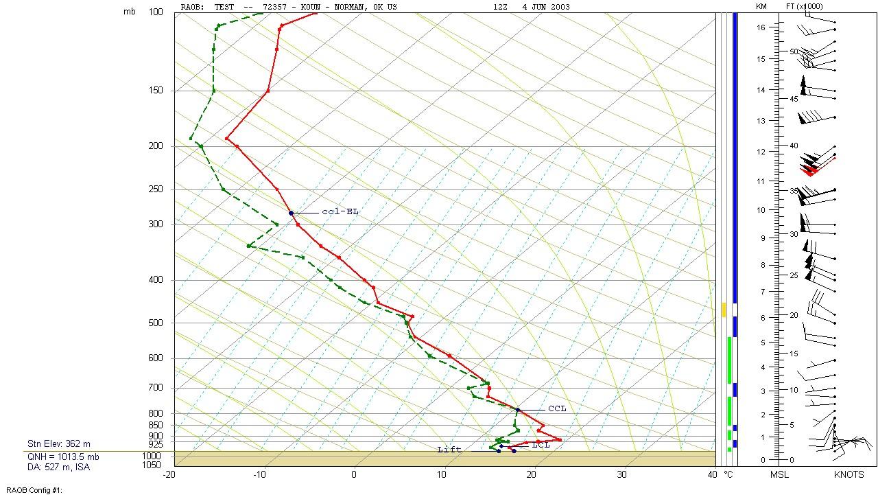 Figure 3.30 12Z KOUN Sounding.
The June 4, 2003 storm is part of the Thunderstorm Electrification and Lightning Experiment (TELEX) taking place in Norman, OK. Radar data for this flight is recorded by the KTLX WSR-88D radar located in Oklahoma City. Upper air soundings for this project are provided by the National Weather Service Field office in Norman Oklahoma (KOUN) and by balloon soundings launched by the project scientists. The Radar and KOUN sounding data are obtained from the NCDC archive and the special project soundings from the TELEX website. The T-28 is based out of the Norman airport for this project.
Top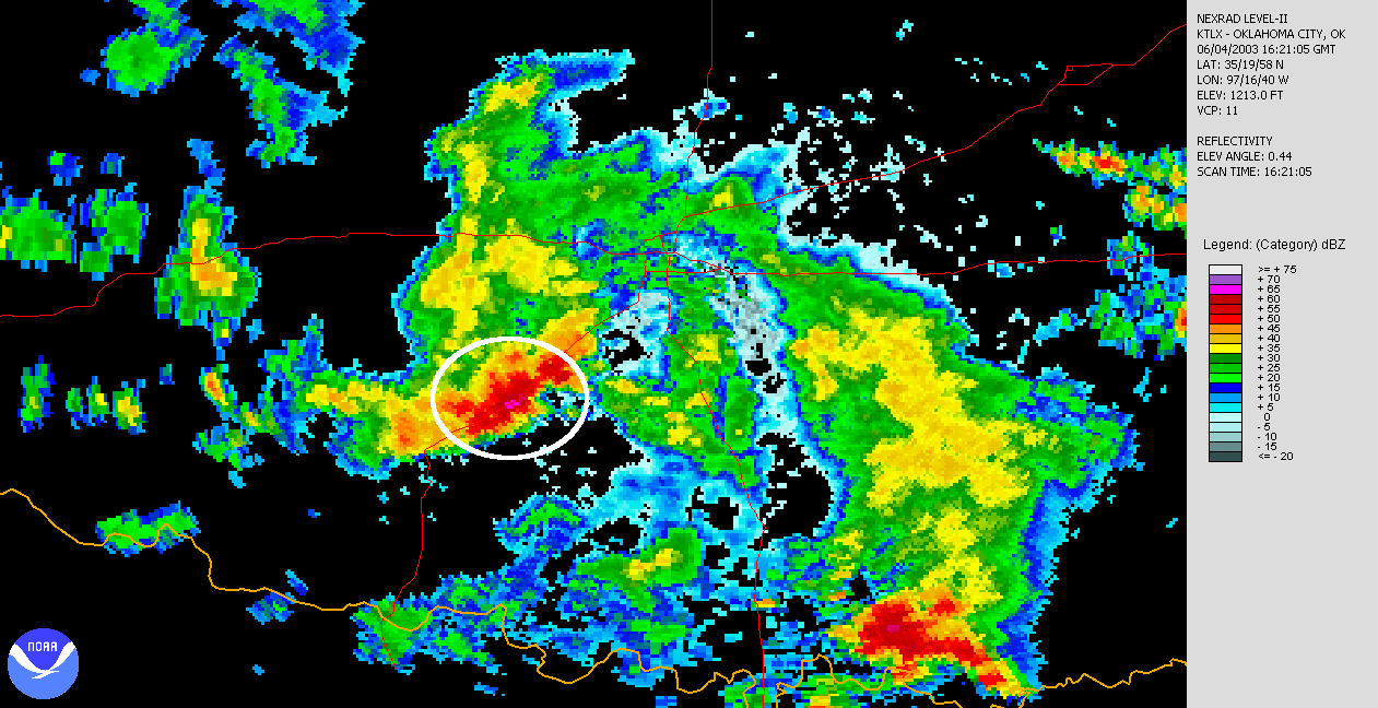 Figure 3.31 0.5 degree base reflectivity scan at 16:21:05
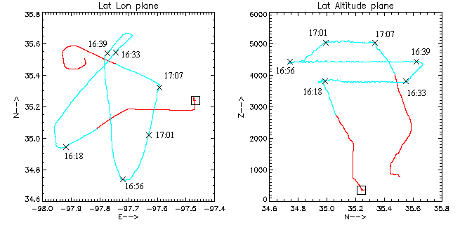 Figure 3.32 Plan view and vertical profile of the T-28 flight track.
According to the project report, the T-28 is launched just before 16:00 UTC on June 4, in the late morning local time. The 12:00 UTC sounding from KOUN plotted in RAOB (Figure 3.30) indicates conditions not indicative of a severe weather day, but the storm under study is a remnant of the previous day's convection that propagated southeastward into the Oklahoma City area. There is strong velocity shear, but very little directional shear. The 0° C level is around 650mb with the CCL at 850 mb, indicating that the storm should contain a mixture of warm rain and supercooled water. An initial 0.5 degree base reflectivity scan in java NEXRAD taken close to the time of take off (Figure 3.31) shows a rather cluttered, unorganized, chaotic structure. In the image, the storms to the west and southwest are passing close to the study area. Active convection appears to be along the southern leading edge with a trailing stratiform region extending northward. The storm summary report indicates that the vertical storm structure indicated that it is more of a rain producing storm. This indicates that very little, if any, hail should be observed.
Analysis of the flight track in T-ADP (Figure 3.32) indicates three distinct passes through the storm. The passes are not obvious in the plan view, but examination of the Latitude-Altitude plane cross section clearly shows the pilot maintained three distinct flight levels. The first pass began at 16:18 and lasted until 16:33, where the pilot maintained an altitude of approximately 3.8 km, with a temperature ranging between 0° C and -2° C. This pass includes penetrating the main convective region and through the trailing stratiform. The second pass runs from 16:39 to 16:56 at an altitude of approximately 4.4 km with a temperature around -3° C and represents a pass through the stratiform region and back into the main convective region. The third and final pass begins at 17:01 and lasts until 17:07 at an altitude of approximately 5 km and with temperature of between -5° C and -6° C. During this pass, the aircraft passes close to the convective region, but stays in the stratiform region for the majority of the flight.
After take off, the aircraft ascended to its initial approach altitude between 16:08 and 16:18. Figure 3.33 is a plot of the temperature profile in RAOB recorded by both instruments on board the T-28 overlaid with a project balloon sounding taken around 16:14. The procedure for producing this plot is the same as in the first case study. The Rosemount and RFT sensors indicate a fairly consistent discrepancy of approximately 2 degrees throughout the ascent. In Figure 3.32, the pilot reports entering cloud during the ascent at approximately 2.8 km. This point is evident as a cusp in both temperature profiles in the T-28 sounding (Figure 3.33). This boundary appears to have no influence on the temperature bias observed between the two instruments. The consistent nature of this difference suggests that the RFT unit has a 2 degree bias and that all observations made with the RFT should be reduced by 2 degrees. Factoring in the two degree bias in the RFT sensor, the overall recorded temperature profile still is a couple of degrees warmer than the balloon sounding. However, this discrepancy fades towards the top of the sounding. The balloon sounding is launched to the northwest of the airport. At this location, the balloon passed through the storm, while the majority of the T-28's climb is performed in clear air away from the storm. This difference in environments could explain the discrepancy between the two soundings.
Top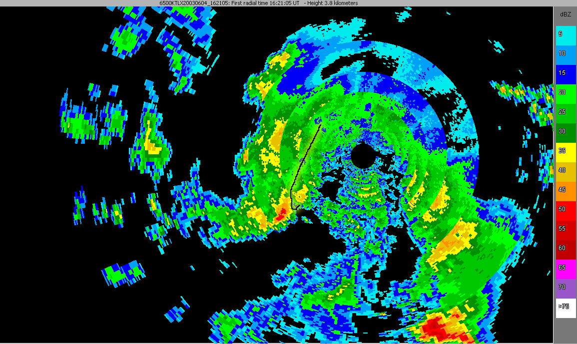 Figure 3.34 3.8 km CAPPI with the T28 flight track overlaid.
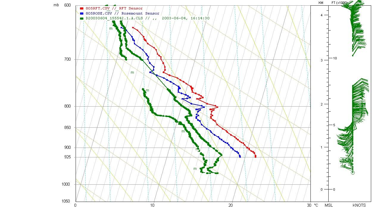 Figure 3.33 Comparison between T-28 and balloon sounding.
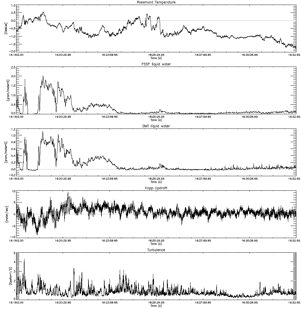 Figure 3.35 Temperature, Liquid Water, updraft and turbulence for pass 1.
Generating an overlay of the flight track on the radar image (Figure 3.34) using IDL and the previously discussed method shows that the first pass begins with the pilot making a right hand turn into the main convective region. He passes through the main convection and continues on into the trailing stratiform region. The radar image in figure 3.34 is a 3.8 km CAPPI reflectivity image at 16:21:05. Due to the slowly changing nature of the storm, this track represents the storm environment encountered by the aircraft during the entire 15 minutes of the penetration fairly accurately. This is determined by examination of an animated radar loop generated with java NEXRAD (not shown). Since the aircraft passes through the main convective region first, the initial portion of the penetration should be marked with the greatest updrafts, most turbulence and largest ice.
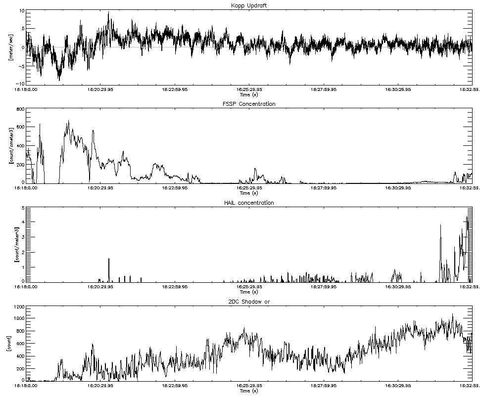 Figure 3.36 Same as Figure 3.35, but showing updraft, FSSP concentration, HAIL concentration and 2DC counts.
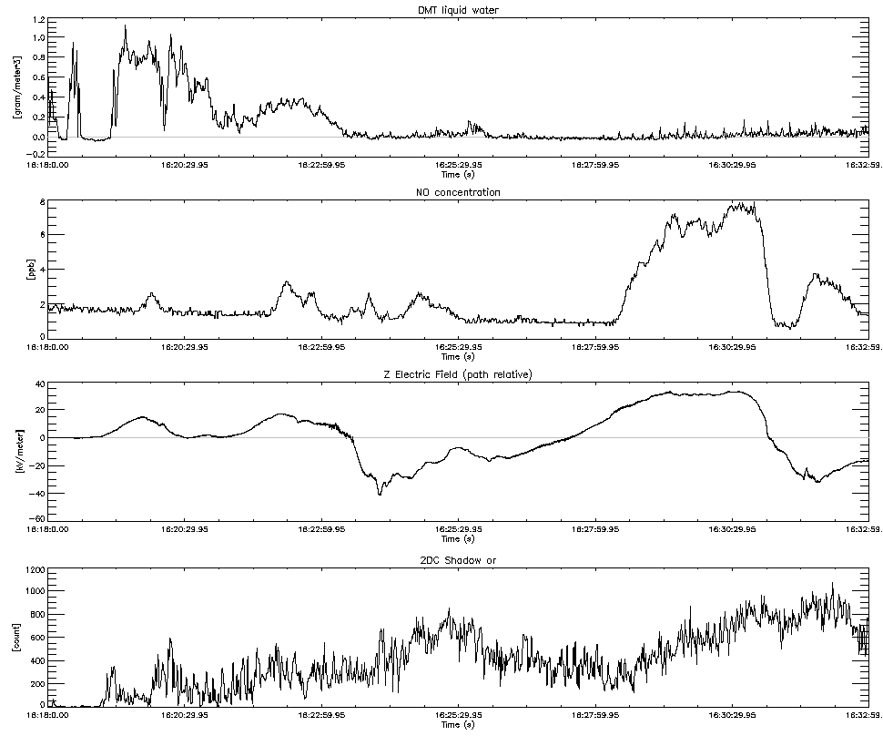 Figure 3.37 Same as Figure 3.35, but showing DMT liquid water, NO concentration, vertical path relative electrical field and 2DC shadow or.
Figures 3.35 illustrates the hydrometeor characteristics found in pass one as well as the updrafts, temperature and turbulence. The initial portion of the pass, after the pilot makes the 30° right turn into the convective region, is marked with elevated liquid water contents shown in both the FSSP and DMT readings. The temperature is also warmer and there is the presence of a stronger updraft. There is indication of a downdraft at the very beginning of the period. It is hard to determine the exact magnitude, as the pilot is in a sweeping turn during this period, but there is a noticeable drop in the FSSP and DMT liquid water contents, and a slight increase in the 2DC counts, indicative of a downdraft region. These findings correlate to the expected findings from the flight track, radar overlay (Figure 3.34), as the aircraft encountered a region of active convection before entering the trailing stratiform region. Closer examinations of the peaks in liquid water content reveal that two peaks are present. There is an initial large peak followed by a smaller one. It is interesting to note that the DMT and FSSP liquid water traces follow very similar curves, but the values do not agree. The FSSP reads the initial peak in liquid water to be on average 1.5 g m-3 while the DMT unit reads an average of 0.8 g m-3. The second peak shows similar behavior with the FSSP liquid water content averaging 0.5 g m-3 while the DMT probe averages 0.3 g m-3. Since the temperature plot indicates that the aircraft is close to or below the melting level, ice contamination in the FSSP is not likely. Since the FSSP estimates liquid water based on accumulated averages of droplet size, small calibration errors tend to accumulate. The DMT, on the other hand, measures cloud liquid water based on fundamental principals. This could be the cause of the discrepancy between the two instruments. Whenever there is a discrepancy between the two probes, the DMT should be assumed to be correct. The elevated 2DC shadow/or counts during this time period (Figure 3.36) are most likely rain drops. There are a few counts from the HAIL probe, but these are most likely caused by liquid water collecting on the probe's arms and streaming past the optics. After these two observed peaks, the liquid water content recorded by both instruments decreases to below 0.2 g m-3 for most of the remainder of the pass. After the liquid water content drops close to zero, the 2DC shadow/or counts continue to climb. This indicates that the aircraft is beginning to encounter ice and snow in the stratiform region of the storm. This is supported by the drop in temperature below 0° C and the lack of liquid water being reported by both the DMT and FSSP. During this period, the DMT does show some variability compared to the FSSP. These small jumps in liquid water are an indicator snow flakes and snow aggregates are striking the DMT's heated element. Both of these observations are consistent with the pilot flying from a region of convective activity into the trailing stratiform region. It is interesting to note that while in the convective region, the pilot experiences a general, uniform updraft; once he is in the non-convective, stratiform region he still experiences variable updrafts and downdrafts, though weak. This could indicate the presence of small scale convection or other mixing processes in the stratiform region of the cloud. But the regular oscillations in updraft more probably indicate an instrumentation artifact with one of the component variables in the updraft calculation. At the end of the period, there is a increase in the hail activity. Brief examination of the 2DC buffers indicate that this is caused by large wet snowflakes being counted as small hail by the hail spectrometer.
The electrical structure of the storm can be examined using the T-28's field mills to generate directional electrical field plots. Figure 3.37 shows the z component of the path relative electric field compared to the DMT liquid water, 2DC shadow/or and nitric oxide concentration. The path relative electric field has axis oriented such that the Z component is normal to the earth's surface. The X and Y axis are parallel to the earth's surface such that the X axis is parallel to the direction of flight. There are two small peaks in vertical electric field corresponding to the two observed updrafts, indicated by the peaks in DMT liquid water. These positive peaks indicate the presence of a negative charge above the aircraft, or a positive charge below. Given the low altitude of the aircraft during this pass, this could be caused by growing graupel higher up in the updraft column which takes on a negative charge. Immediately after exiting the updraft region, the vertical electric field drops into the negative, indicating a positive overhead charge or a negative charge underneath. Positive charge overhead could be producing the strong negative field. It could be caused by positively charged ice crystals being advected out of the top and away from the updraft. This is consistent with the idea that the storm has a classic normal dipole structure with positive charge at the cloud top and negative charge at the base. Further on, the field reverses again for a short time. Since this portion of the storm did not show convective activity in the radar scans, any elevated negative charge would have to come from leftover ice from decaying cells. This could be possibly caused by an inverted dipole layer described by Funk (2002).
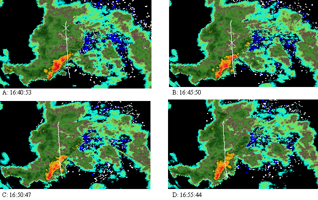 Figure 3.38 Flight track for pass 2 overlaid on 0.5 degree base reflectivity scans
The nitric oxide plot indicates peaks in NO correlating to changes in electric field. Even where the ambient field is negative, there is a noticeable increase in the electric field corresponding to peaks in NO concentration. The increase in NO concentration seems reasonably well correlated with the vertical electric field, as higher peaks in field strength relate to higher peaks in NO concentration and the width of the NO concentration peaks span the same width as the elevated field readings. The strong correlation of NO to electric field is puzzling. Since NO is produced by lightning channels, natural NO readings should look like small jumps in concentration, corresponding to crossing an old strike channel, or possibly broad regions of low concentration due to mixing of NO created by multiple discharges. In Figure 3.37, it appears that there is a critical absolute electric field value of approximately 15 kv m-2 that must be reached before NO is observed. This indicates that the NO is most likely being produced by some other mechanism, possibly associated with the sampling inlet or some other part of the aircraft itself. This warrants further investigation.
Top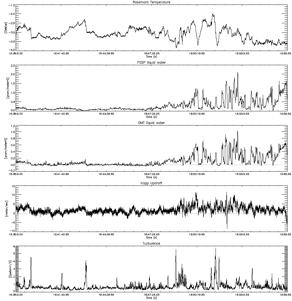 Figure 3.39 Same as figure 3.35 except for pass 2
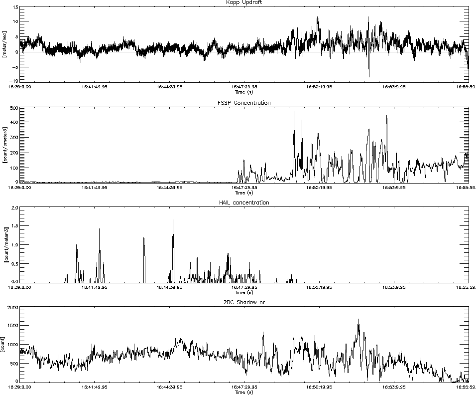 Figure 3.40 Same as figure 3.36 except for pass 2
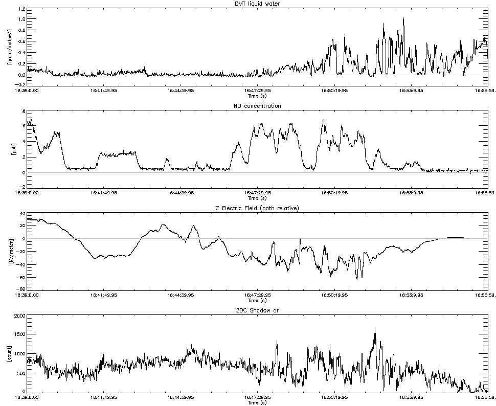 Figure 3.41 Same as figure 3.37 except for pass 2
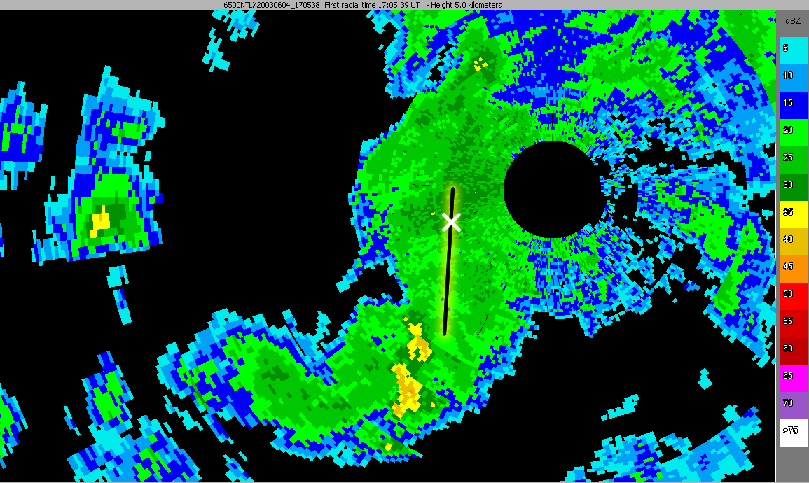 Figure 3.42 5 km CAPPI with T-28 flight track overlaid.
The second pass in the storm involves the aircraft returning through the stratiform region and reentering the convective region. Figure 3.38 shows the progression of the plane through the storm at the four radar sweep times. Analysis of a 4.4 km CAPPI (not shown) reveals little difference between it and the 0.5 degree base reflectivity. According to Figure 3.37, the aircraft enters the main convective region sometime between 16:45:50 and 16:50:47 and then exits the region around 16:55:44.
Figure 3.39 shows the temperature, updraft and particle data for the pass. The beginning of the pass is marked by low liquid water contents, recorded by both the DMT and FSSP, and elevated 2DC counts. During this time, there also appears to be an elevated concentration of larger particles being picked up by the HAIL spectrometer. Except for the increase in aggregates, the observed pattern is the same as observed in the last half of the previous region identified as stratiform cloud. The values of liquid water content and 2DC counts for this region match with those recorded during the first pass fairly closely, indicating a fairly homogeneous layer. The in cloud temperature in this region of the storm is lower than the first pass, with temperatures now well below -2 degrees C. This is expected as the aircraft is approximately 600 m higher in elevation than the previous pass. The stratiform region of this pass also contains regions of weak updrafts and downdrafts. It is interesting to note that at this higher altitude, the magnitude of the vertical motions is greater and accompanied by greater turbulence. There are several weak, but notable updrafts that correspond to regions of elevated turbulence and small peaks in liquid water. The peaks in liquid water are, however, small and only show up in the DMT liquid water trace, indicating they are most likely due to individual snow particles hitting the heated coil. The increase in concentration of larger particles being picked up by the HAIL spectrometer probe is interesting, especially compared to almost nonexistent observations from the first pass. These elevated concentrations could again be from larger aggregates.
At the end of the pass, the aircraft enters the convective region of the storm again. This is clearly seen in Figure 3.39 as an increase in FSSP and DMT liquid water, stronger updrafts and elevated turbulence. As observed in the previous pass, the FSSP liquid water content is reading consistently higher than the DMT liquid water, possibly from the previously discussed faulty size calibration. A major difference between this pass and the last one is in the 2DC data in Figure 3.40. In the previous pass, there are few particles being picked up by the 2DC in the convective region. However, in this pass, there are quite a few. There is a distinct decline in the number of particles as the aircraft leaves the stratiform region, but there are several peaks observed which are well correlated with peaks in FSSP concentration.
The vertical (Z) electric field plot in Figure 3.41 indicates that the vertical electric field for the majority of the pass is negative, indicating a positive charge layer above or, less likely, a negative charge layer below. There are two locations within the first half of the flight where there is a positive field, indicating a negative charge layer above the aircraft or a strong positive layer below the aircraft. This could possibly be the inverted dipole structure implied in the first pass. Unlike the first pass, there appears to be no solid correlation between the vertical electric field patterns and the updraft region (indicated by DMT liquid water). Nitric oxide concentration does correlate well with the observed negative field around 16:41:50 and with the larger region of negative field associated with the elevated 2DC records. At the end of the pass, the electric field approaches zero, which is expected as the flight track indicates the aircraft exiting the cloud. It is interesting to note that the DMT liquid water content (Figure 3.39) and the FSSP concentration (Figure 3.40) both increase at the very end of the pass when the aircraft exists the radar echo. During this time, the 2DC shadow or indicates almost no activity, indicating that the aircraft is passing through a small, non-glaciated tower that has an echo too weak to show up on radar. The lack of ice in the 2DC plot and the zero vertical electric field both indicate that the cloud is mostly cloud liquid water and has not yet begun to form rain or grapple.
Top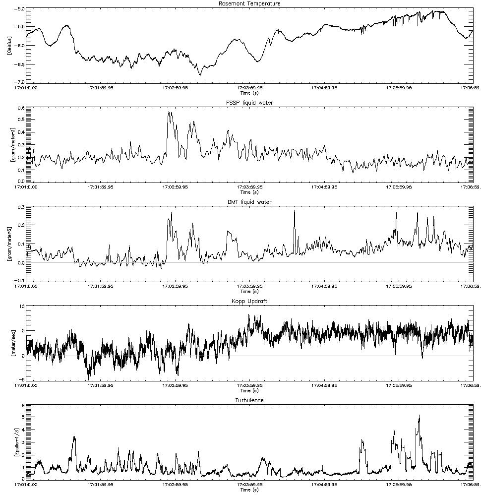 Figure 3.43 Same as figure 3.35 except for pass 3
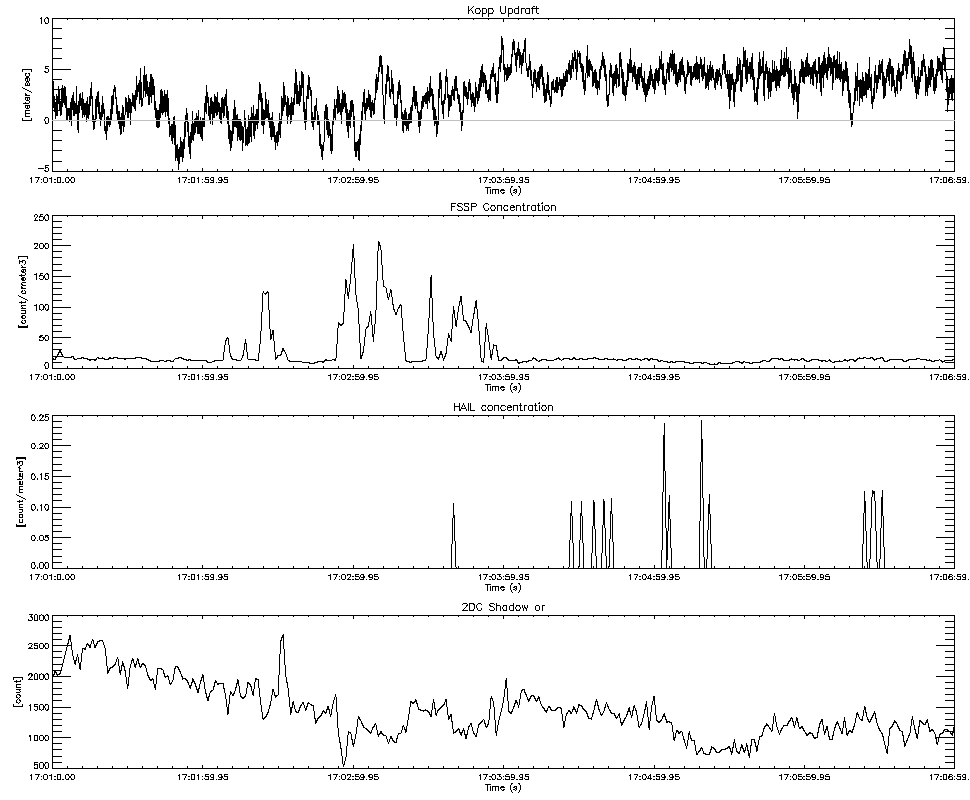 Figure 3.44 Same as figure 3.36 except for pass 3
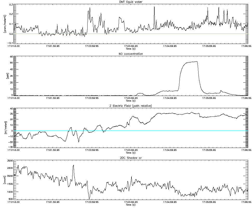 Figure 3.45 Same as figure 3.37 except for pass 3
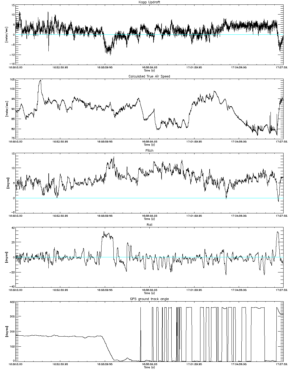 Figure 3.46 Diagnostic plots of aircraft motion variables
The third and final pass through the storm involves the aircraft climbing to 5 km and returning to the north through the stratiform region of the storm. The track of the aircraft overlaid with a 5 km CAPPI is presented in Figure 3.42. The white X indicates the aircraft's position at the time the scan is completed. The radar image indicates the presence of convective activity towards the beginning of the pass and benign stratiform echoes for the remaining majority. This observation is consistent with the structure observed in the previous two passes.
Figure 3.43 shows the liquid water properties with temperature, updraft, and turbulence. The updraft profile for this pass shows the exact opposite of what is expected. In the initial portion of the pass, which is close to the region of convection, there is evidence of a definite updraft and downdraft followed by sporadic regions of updraft and downdraft. This is consistent with previous observations within the convective region. Once in the stratiform region, the aircraft begins to encounter a constant updraft. This observation is different from the previous two passes which experienced relatively weak vertical motions in the stratiform region. The DMT liquid water profile seems to confirm the presence of the updraft in the stratiform region, showing elevated readings beginning around 17:03. The 2DC Shadow or plot in Figure 3.44 indicates the presence of a large concentration of small ice, rain drops or graupel in the convective region, but concentrations taper off as the aircraft moves out of the region. This is the reverse of the pattern observed in the previous two flights.
In comparison to the other passes, the 2DC counts for the convective region of pass 3 are greatly elevated. The observed lower readings in the stratiform region are actually very similar to the readings in the stratiform region of the previous flights. This indicates that stratiform region may contain the same amount of ice as in previous passes, but the convective region now contains more, larger particles. The CAPPI (Figure 3.42) indicates that the convective region contains much lower echo intensity than lower regions of the storm at the same position. Since the aircraft is now at 5 km, the aircraft is most likely in the middle portion of the collapsing updraft,. The updraft and downdraft regions are evident in the updraft plot (Figure 3.43) just before 17:02 with a corresponding spike in turbulence at the transition point. There is no appreciable difference in any of the hydrometeor variables delimiting the updraft or downdraft except in the DMT liquid water, which shows very low values in the downdraft region. This same feature is not observed in the FSSP or 2DC plots, as these two instruments are being overwhelmed with small ice particles. The vertical electric field (Figure 3.45) observed in the convective region is primarily negative, indicating the presence of a negative charge layer below the aircraft, a positive charge layer above the aircraft or a combination of both. The previous passes have substantiated that the storm has a normal dipole. However, in the more convective region a negative field would most likely be caused by a negative charge on precipitation that has fallen below the aircraft.
The updraft observed in the stratiform region of the storm is not intuitive. There are no strong echoes on the 5 km CAPPI to indicate a region of updraft. Figure 3.43 indicates that in the latter part of the broad indicated updraft there is significantly increased turbulence and the DMT probe suggests elevated liquid water, both of which are consistent with an updraft. However, the FSSP concentration plot (Figure 3.44) shows no increase in particles, as is observed with the previous elevated liquid water content associated with the convective region. As discussed earlier, the 2DC shadow/or plot also indicates similar counts to the previous passes through the stratiform region that did not display this constant updraft. Review of the updrafts observed in passes one and two also reveal slightly suspect updraft records. Figure 3.46 shows a diagnostic of the updraft by comparing some variables used in the calculation along with the GPS ground track angle. This plot is from 16:50:00 to 17:08:00 to compare the air speed and updraft values to a longer record. Since the suspect updraft consumes a large portion of the time period of pass 3, expanding the time range introduces more data and gives a better comparison. In this plot, the ground track indicates fairly straight flight. The jumpiness of the plot is due to the discontinuity of the compass dial at true north. The pitch and roll data do not show a significant difference during the updraft region in question. The only noticeable difference is a drop in airspeed of approximately 15 m s-1. Review of the Kopp updraft equation reveals that the updraft calculation is only valid for a 'normal penetration speed.' This artificial updraft is an artifact of the aircraft no longer flying at 'normal penetration speed.'
Between 17:05 and 17:06 there is a strong peak in NO concentration. This peak is actually a calibration tests being performed by the pilot and is indicated in the pilot report. In this test, the air supply tube to the NO monitor is switched to a tube connected to a bag containing air with 50 ppb NO. The recorded reading of 50 ppb NO indicates that the instrument is well within calibration.
TopThe organization of this flight is different from the first storm in the study. Analysis of the plan view flight track did not reveal a clear breakdown of the flight into passes. However, the cross sections helped greatly in determining how to divide up the storm. This flight is an example of a situation where the passes are not directly after one another. The aircraft took several minutes to climb to the new altitude and set up before starting the next pass. Data from these interim periods is not considered in this study, as updraft data would be severely contaminated by the banking turns and the main focus is to observe the transition from the convective region to the stratiform region. There still exists viable data in these regions, but it is deemed unnecessary for this study. The data archive contains over 100 different variables recorded at least every second for a period lasting an hour or more. There is realistically too much data for a single study to focus on every point and aspect of it, and being able to limit the analysis is crucial.
In this flight, the nature of the penetration is such that the aircraft experienced the same parts of the storm at different altitudes. This type of situation is best suited to develop a virtual cross section. In each pass, the same variables are analyzed and the key features are picked out and diagnosed. This approach requires the user to take a synergistic approach not only when comparing different plots from the same pass, but mentally visualize the three dimensional extent of the data.
The updraft artifact observed in the final section of the pass also raises an important point about data integrity. As discussed previously, the data in the archive is not completely free from error. On first glance, the updraft artifact raises alarm bells, as nothing in any of the conceptual models predicts that kind of steady updraft. The updraft is also too 'perfect.' When reading data of this nature, prolonged features like that are not common and the unnatural appearance of it should mark it for further investigation. In this case, researching the algorithm used to calculate the updraft variable and analyzing the components individually revealed the culprit constituent. When conducting an analysis of this nature, it is important to follow through with diagnosing artifacts in this fashion. The archive contains a large collection of variables that can be used for diagnostic measures, and the supporting web site contains the information on the instruments and needed to critically decide if a feature in the data is an artifact or an actual feature worthy of further exploration.
Top