NEARLY FINAL.

Table of Contents

• Introduction
• Data Access
• Location
• Photographs
• Sensors
• Table of Variables
• Processing Notes
• Daily Weather Plots
• Other Plots

Introduction

Data Access

• 5-minute averages of first and second-order moments of calibrated data. We recommend combining these to obtain more statistically-significant averages over longer time periods. These are available in NetCDF data files.

A complete list of variables is available. This list shows the NetCDF variable name, dimensions, descriptive variable name, units, and additional comments, if available. Each file contains all the statistics for one day, beginning at 00:00:00 UTC. Most variables are dimensioned (time, station), where time is in 5 minute increments (288 per day), station is 1 or 2 for variables common to NCAR (station=1) and Oklahoma (station=2). Variables without a station dimension were measured by either NCAR or OK, but not both. See the Sensors description below for guidance as to where the variables were measured.

Most descriptive variable names hopefully are self-explanatory. Those beginning with Capital letters came from slow response sensors and those with lower cases letters from fast response sensors. Higher order statistics are indicated by products of variables. For example, w'tc' is the covariance between vertical velocity and sonic virtual temperature and h2o'h2o'h2o'h2o' is the fourth order moment of water vapor mixing density. For some variables, the sensor name is appended, e.g. "v.nuw1" is the lateral velocity component from the one of the new sonic anemometers we built with a University of Washington-style array, to distinguish it from "v" which is the same variable measured by other sonic anemometers.

Location

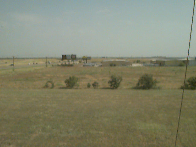
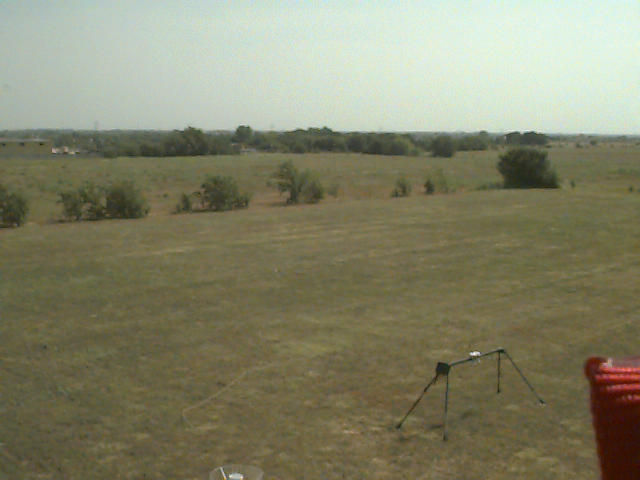
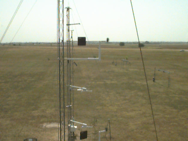
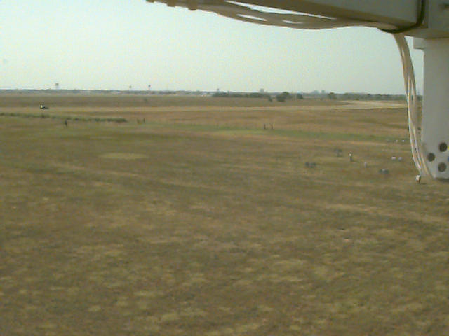
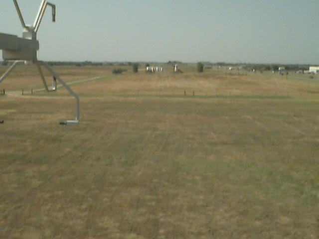
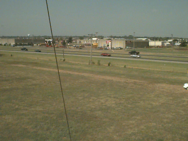
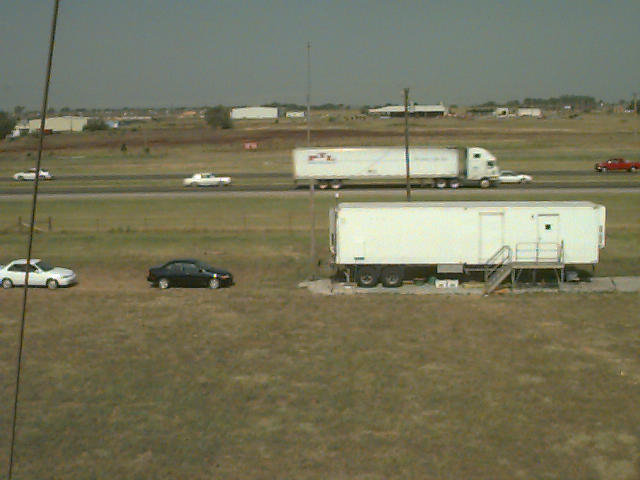
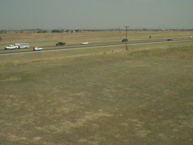
A series of views forming a panorama from the 9m level of the sonic tower is available here:

1. North
2. Northeast
3. East
4. Southeast
5. South
6. Southwest
7. West
8. Northwest

Photographs

The data files contain data from NCAR and the University of Oklahoma Mesonet. The NCAR sensors are mostly described in the ASTER Facility Description. A color-coded diagram of the variables from these sensors was created to help sort out the variables.

Table of Variables

Variable Name	Description	Units	Dimension	Sensor	Notes
base_time	Seconds since 1970 Jan 1 00:00 GMT	seconds
time	Seconds since base_time	seconds	time
Gsoil.5cm.1	Soil Heat Flux	W/m^2	time x station
Gsoil.5cm.2	Soil Heat Flux	W/m^2	time x station
Gsoil.5cm.3	Soil Heat Flux	W/m^2	time
Mp.5cm.1		msec	time
Mp.5cm.2		msec	time
Mp.5cm.3		msec	time
Msoil.5cm.1	Soil Moisture	V frctn	time x station
Msoil.5cm.2	Soil Moisture	V frctn	time
Msoil.5cm.3	Soil Moisture	V frctn	time
P	Barometric Pressure	mb	time x station
RH.0.5m	Rel. Humidity	%	time
RH.1.5m.2	Rel. Humidity	%	time
RH.1.5m.3	Rel. Humidity	%	time
RH.1.5m	Rel. Humidity	%	time x station
RH.4.5m	Rel. Humidity	%	time
RH.6.5m	Rel. Humidity	%	time
RH.9m	Rel. Humidity	%	time x station
Rlw.in.CNR1a	Incoming Longwave	W/m^2	time
Rlw.out.CNR1a	Outgoing Longwave	W/m^2	time
Rnet.CNR1a	Net Radiation	W/m^2	time
Rnet.NRLite.3	Net Radiation	W/m^2	time
Rnet	Net Radiation	W/m^2	time x station
Rpile.in.CNR1a	Up-looking Thermopile	W/m^2	time
Rpile.in	Up-looking Thermopile	W/m^2	time x station
Rpile.out.CNR1a	Down-looking Thermopile	W/m^2	time
Rpile.out	Down-looking Thermopile	W/m^2	time x station
Rsw.in.CNR1a	Incoming Shortwave	W/m^2	time
Rsw.in	Incoming Shortwave	W/m^2	time x station
Rsw.out.CNR1a	Outgoing Shortwave	W/m^2	time
Rsw.out	Outgoing Shortwave	W/m^2	time x station
Spd.2m	Wind Speed	m/s	time x station
Spd.9m	Wind Speed	m/s	time x station
T.0.5m	Air Temp	degC	time
T.1.5m.2	Air Temp	degC	time
T.1.5m.3	Air Temp	degC	time
T.1.5m	Air Temp	degC	time x station
T.4.5m	Air Temp	degC	time
T.6.5m	Air Temp	degC	time
T.9m	Air Temp	degC	time x station
Tadam.marigold	Electronics Temp	degC	time
Tadam.ragwort	Electronics Temp	degC	time
Tcase.CNR1a		W/m^2	time
Tcase.in	Up-looking Case Temp	degC	time x station
Tcase.out	Down-looking Case Temp	degC	time x station
Tdome.in	Up-looking Dome Temp	degC	time x station
Tdome.out	Down-looking Dome Temp	degC	time x station
Tsfc	Surface Temp	C	time
Tsoil.5cm.1	Soil Temperature	degC	time x station
Tsoil.5cm.2	Soil Temperature	degC	time x station
Tsoil.5cm.3	Soil Temperature	degC	time
U.10m	Eastward Wind	m/s	time
U.1m	Eastward Wind	m/s	time
U.2m	Eastward Wind	m/s	time
U.4.5m	Eastward Wind	m/s	time
U.6.5m	Eastward Wind	m/s	time
U.9m	Eastward Wind	m/s	time
V.10m	Northward Wind	m/s	time
V.1m	Northward Wind	m/s	time
V.2m	Northward Wind	m/s	time
V.4.5m	Northward Wind	m/s	time
V.6.5m	Northward Wind	m/s	time
V.9m	Northward Wind	m/s	time
cflag.nuw1			time
cflag.nuw2			time
diag.csat			time
h2o'h2o'.4.5m	h2o variance	(g/m^3)^2	time x station
h2o'h2o'.9m	h2o variance	(g/m^3)^2	time
h2o.4.5m	Water Vapor Density	g/m^3	time x station
h2o.9m	Water Vapor Density	g/m^3	time
lev.rad.x		deg	time
lev.rad.y		deg	time
lev.u.4.5m		deg	time
lev.u.9m		deg	time
lev.v.4.5m		deg	time
lev.v.9m		deg	time
mr'mr'.bph.4.5m		(gm/kg)^2	time
mr.bph.4.5m		gm/kg	time
raina	Rain Accumulation	mm	time x station
rainr	Rain Rate	mm/hr	time x station
rh.bph.4.5m		%	time
t't'.4.5m	t variance	(degC)^2	time x station
t't'.bph.4.5m	t variance	(degC)^2	time
t.4.5m	Air Temperature	degC	time x station
t.bph.4.5m	Air Temperature	degC	time
tc'tc'.4.5m	tc variance	(degC)^2	time x station
tc'tc'.9m	tc variance	(degC)^2	time
tc'tc'.csat	tc variance	(degC)^2	time
tc'tc'.nuw1	tc variance	(degC)^2	time
tc'tc'.nuw2	tc variance	(degC)^2	time
tc.4.5m	Virtual Temperature	degC	time x station
tc.9m	Virtual Temperature	degC	time
tc.csat	Virtual Temperature	degC	time
tc.nuw1	Virtual Temperature	degC	time
tc.nuw2	Virtual Temperature	degC	time
tcflag.4.5m	Spike fract for tc		time
tcflag.9m	Spike fract for tc		time
tcflag.csat	Spike fract for tc		time
u'h2o'.4.5m	u h2o covariance	m/s g/m^3	time x station
u'h2o'.9m	u h2o covariance	m/s g/m^3	time
u'mr'.(,bph).4.5m		m/s gm/kg	time
u't'.(,bph).4.5m	u t covariance	m/s degC	time
u't'.4.5m	u t covariance	m/s degC	time x station
u'tc'.4.5m	u tc covariance	m/s degC	time x station
u'tc'.9m	u tc covariance	m/s degC	time
u'tc'.csat	u tc covariance	m/s degC	time
u'tc'.nuw1	u tc covariance	m/s degC	time
u'tc'.nuw2	u tc covariance	m/s degC	time
u'u'.4.5m	u variance	(m/s)^2	time x station
u'u'.9m	u variance	(m/s)^2	time
u'u'.csat	u variance	(m/s)^2	time
u'u'.nuw1	u variance	(m/s)^2	time
u'u'.nuw2	u variance	(m/s)^2	time
u'v'.4.5m	u v covariance	(m/s)^2	time x station
u'v'.9m	u v covariance	(m/s)^2	time
u'v'.csat	u v covariance	(m/s)^2	time
u'v'.nuw1	u v covariance	(m/s)^2	time
u'v'.nuw2	u v covariance	(m/s)^2	time
u'w'.4.5m	u w covariance	(m/s)^2	time x station
u'w'.9m	u w covariance	(m/s)^2	time
u'w'.csat	u w covariance	(m/s)^2	time
u'w'.nuw1	u w covariance	(m/s)^2	time
u'w'.nuw2	u w covariance	(m/s)^2	time
u.4.5m	Sonic U Wind Comp	m/s	time x station
u.9m	Sonic U Wind Comp	m/s	time
u.csat	Sonic U Wind Comp	m/s	time
u.nuw1	Sonic U Wind Comp	m/s	time
u.nuw2	Sonic U Wind Comp	m/s	time
uaflag.nuw1		G	time
uaflag.nuw2		G	time
uasamples.nuw1			time
uasamples.nuw2			time
ubflag.nuw1			time
ubflag.nuw2			time
ubsamples.nuw1		G	time
ubsamples.nuw2		G	time
ucflag.nuw1			time
ucflag.nuw2			time
ucsamples.nuw1		G	time
ucsamples.nuw2		G	time
uflag.4.5m	Spike fract for u	G	time
uflag.9m	Spike fract for u	G	time
uflag.csat	Spike fract for u		time
usamples.4.5m	# of samples averaged	G	time
usamples.9m	# of samples averaged	G	time
v'h2o'.4.5m	v h2o covariance	m/s g/m^3	time x station
v'h2o'.9m	v h2o covariance	m/s g/m^3	time
v'mr'.(,bph).4.5m		m/s gm/kg	time
v't'.(,bph).4.5m	v t covariance	m/s degC	time
v't'.4.5m	v t covariance	m/s degC	time x station
v'tc'.4.5m	v tc covariance	m/s degC	time x station
v'tc'.9m	v tc covariance	m/s degC	time
v'tc'.csat	v tc covariance	m/s degC	time
v'tc'.nuw1	v tc covariance	m/s degC	time
v'tc'.nuw2	v tc covariance	m/s degC	time
v'v'.4.5m	v variance	(m/s)^2	time x station
v'v'.9m	v variance	(m/s)^2	time
v'v'.csat	v variance	(m/s)^2	time
v'v'.nuw1	v variance	(m/s)^2	time
v'v'.nuw2	v variance	(m/s)^2	time
v'w'.4.5m	v w covariance	(m/s)^2	time x station
v'w'.9m	v w covariance	(m/s)^2	time
v'w'.csat	v w covariance	(m/s)^2	time
v'w'.nuw1	v w covariance	(m/s)^2	time
v'w'.nuw2	v w covariance	(m/s)^2	time
v.4.5m	Sonic V Wind Comp	m/s	time x station
v.9m	Sonic V Wind Comp	m/s	time
v.csat	Sonic V Wind Comp	m/s	time
v.nuw1	Sonic V Wind Comp	m/s	time
v.nuw2	Sonic V Wind Comp	m/s	time
vflag.4.5m	Spike fract for v		time
vflag.9m	Spike fract for v		time
vflag.csat	Spike fract for v		time
vsamples.4.5m	# of samples averaged	G	time
vsamples.9m	# of samples averaged	G	time
w'h2o'.4.5m	w h2o covariance	m/s g/m^3	time x station
w'h2o'.9m	w h2o covariance	m/s g/m^3	time
w'mr'.(,bph).4.5m		m/s gm/kg	time
w't'.(,bph).4.5m	w t covariance	m/s degC	time
w't'.4.5m	w t covariance	m/s degC	time x station
w'tc'.4.5m	w tc covariance	m/s degC	time x station
w'tc'.9m	w tc covariance	m/s degC	time
w'tc'.csat	w tc covariance	m/s degC	time
w'tc'.nuw1	w tc covariance	m/s degC	time
w'tc'.nuw2	w tc covariance	m/s degC	time
w'w'.4.5m	w variance	(m/s)^2	time x station
w'w'.9m	w variance	(m/s)^2	time
w'w'.csat	w variance	(m/s)^2	time
w'w'.nuw1	w variance	(m/s)^2	time
w'w'.nuw2	w variance	(m/s)^2	time
w.4.5m	Sonic W Wind Comp	m/s	time x station
w.9m	Sonic W Wind Comp	m/s	time
w.csat	Sonic W Wind Comp	m/s	time
w.nuw1	Sonic W Wind Comp	m/s	time
w.nuw2	Sonic W Wind Comp	m/s	time
wflag.4.5m	Spike fract for w		time
wflag.9m	Spike fract for w		time
wflag.csat	Spike fract for w		time
wsamples.4.5m	# of samples averaged	G	time
wsamples.9m	# of samples averaged	G	time

General

Temperature-Humidity Sensors

Propeller-vane Anemometers

Note that small wind direction differences were observed during the field program which were tracked down to the vanes being slightly bent. Once this problem was identified, some of the vanes were flipped (upside-down) to make the directions more consistent. Again, no attempt to correct the data was made (since it would be very difficult to model this effect and the error is smaller than the accuracy needed for wind directions for this program). See the logbook for details of this problem.

Sonic Anemometers

The new UW sonic anemometers spiked much worse (5-10%; probably due to the longer pathlength). Furthermore, nuw1 developed a transducer problem on 7/26, and nuw2 stopped reporting data on 8/5. These problems are being investigated. The geometry for both arrays was measured on 10/6/98 and found to be within 1 degree of specifications. The new angles have been used in post-processing of the data.

Tilt corrections have been calculated for all of the sonic anemometers using our standard algorithm. These corrections have been applied to all of the statistics in the data files (including those from the Oklahoma Mesonet CSAT sonic anemometer). The maximum "lean" angle found was 1.9 degrees, and most were less than 1 degree, which is typical for a nearly flat site. The values used are:

# yr mon day hh:mm(GMT) lean    leanaz  woffset

4.5m.OKMN:
98 6 23 00:00   0.642   176.3   0.018

4.5m.NCAR:
98 6 17 00:00   1.239   25.3    0.006
# Releveled using bubble level
98 6 29 14:30   0.316   -146.9  -0.022

9m.NCAR:
98 6 17 00:00   0.693   27.4    -0.017
# After v transducer replacement
98 7 10 00:00   1.908   20.5    -0.023

nuw1:
98 7 15 00:00	0.771   -26.6
# After rotating
98 7 24 15:00	0.882   -74.0
# Sensor goes bad (path a transducer?)
98 7 26 12:00   0       0       0

nuw2:
98 7  1 00:00   0.300   27.6
# after flipping and rotating 
# (179.3 = 180.0-0.6 and -177 = 2.7 - 180, to compensate for flip)
98 7 24 15:00	179.341 -177.3

Radiometers

Soil Properties

Daily Weather Plots

June

				18	19	20
21	22	23	24	25	26	27
28	29	30	.	.	.	.

July

			1	2	3	4
5	6	7	8	9	10	11
12	13	14	15	16	17	18
19	20	21	22	23	24	25
26	27	28	29	30	31	.

August

						1
2	3	4	5	6	7	8

Other plots

ATI/CSAT Comparison

NUW Comparison

If anything, the flipped and rotated comparision looks better than for the parallel configuration. This may be due to the arrangement of the supporting booms. The sonic arrays were closer together (and thus would have affected each other over a wider range of wind directions) for the parallel configuration than for flipped and rotated. However, in both cases directions from about 110 to 250 through 180 should have been okay. This still doesn't explain the apparent variation of the parallel data - perhaps the tilt correction was confused by the distortion from the sides and should be recomputed.

Also, the flipped and rotated data show a consistent speed difference (nuw2 higher by 2%). During this period, the Tc values also are higher from nuw2 by 4C (1.3%). Since u~Tc(t1-t2)/2d, about half of the error is explained by how the sensors were zeroed. I'm not sure why this 4C error occurred.

In any case, I would conclude that these arrays do not appear to have flow distortion (no flow distortion correction has been applied to these data) which is evident from this test.

[an error occurred while processing this directive]
This page was prepared by Steven Oncley, NCAR Research Technology Facility