Steps In MTP Post-Campaign Data Analysis
MJ Mahoney
7. Determine OATnavCOR
OATnavCOR is defined as the temperature correction which must be ADDED
to the measured outside air temperature (Tnav) to make it agree with
radiosondes (Traob) that the aircraft flew close to; that is, OATnavCOR
= Traob - Tnav. OATnavCOR is positive if Tnav is colder than
radiosondes, and negative if Tnav is warmer than radiosondes.
Generally, it is unlikely that a radiosonde launch site
will be flown by when the sonde is launched, and in any event, it could
take up to 2 hours for a sonde to reach maximum altitude, so temporal
coincidence is not ever the case. Therefore, when we use sondes to
calibrate the flight level OAT, we must interpolate temporally between
two
soundings. In addition, we examine the two earlier and later soundings
to get a sense of the temporal variability of the air. If it is
substantial, that particular site cannot be used for temperature
calibration. In addition to the temporal variability, we must also be
concerned about the presence of spatial temperature gradients when the
aircraft does not fly close to a particular sonde launch site.

Figure 1. Temperature bias with
range during the SOLVE-2 campaign.
This is illustrated in Figure 1
for the SOLVE-2 flights on January 12, 16, 19, and 21, 2003. To
generate this figure, we compared the temperature on level flight legs
at 35, 39 and 41 kft over distances ranging from 0 to 220 km. Note that
the error bars increase with distance both because of spatial
gradients, but also because there are fewer samples and hence poorer
statistics. It is evident that at FL390 an absolute bias of ~0.5 K can
be expected on average over a distance of 225 km with ~0.5 K standard
deviation (white trace and error bars in Figure 1).
If the aircraft does not fly close to a radiosonde launch site, we
should perform a spatial interpolation between two sound launch sites
(after the temporal interpolation at each of the sites). RAOBman
allows this to be done manually, but this is rather tedious. The
temporal interpolation can also be done manually, but because it was
also tedious, it has been completely automated. Now dozens of temporal
comparisons between MTP retrievals and radiosondes can be performed in
minutes.
Although determination of OATnavCOR only requires comparison of
measured flight level temperatures with nearby radiosonde temperatures
at flight level, we in fact compare the entire retrieved altitude
temperature profile (ATP) to the radiosonde temperature profile. The
reason for doing this is to be able to evaluate the accuracy of the
retrievals above or below flight level. It is very important in this
process to be completely objective in selecting which radiosondes
should be used. The question of objectivity will be discussed further
below.
To perform the RAOB and ATP comparison, a number of files are used:
- MISSION_RAOBSs.RAOB2 - the sorted radiosondes from the last step
that contain all the soundings needed to perform temporal and spatials
interpolations at aircraft flyby times
- MISSION_RAOBused.RAOB2 - a output version of the previous file
containing only those sounding that were actually used. They will
differ if extra before and after soundings are included to study
temporal variations (as they should be!).
- MISSION_RAOBrangeAll.txt - the file containing the time of all
the flybys as well as the LR1, LR2 and Zb estimates.
- RAOBcomparison.txt - the output file from the RAOB/ATP comparison

Figure 2. The RAOBman Blend tab.
Before proceeding with the comparison we need to specify a number of
options on the RAOBman Blend tab, which is shown in Figure 2. These options are all in
the lower right side of the tab and default values are normally "safe"
to use.
- Layer Thickness [m] -
besides doing a direct flight level comparison of OAT, a comparison is
also possible through a specified layer thickness. The reason for doing
this is that a radiosonde may show a lot of variability under some
circumstances, so this has the effect of averaging out the variations.
- Cycles Averaged - the
number of temperature profiles averaged before the comparing to the
RAOB.
- Max Range [km] - the
maximum range of the flyby to be used in comparisons. This allows a
large range to be used when the MISSION_RAOBrangeAll.txt file is
created, but a smaller one to be used when comparisons are made.
- Delta Zp [m] - how much
the aircraft's pressure altitude is allowed during the comparison
cycles. This avoids comparisons, for example, during ascent or descent.
The program will reset and try again if this threshold is exceeded.
- Min Zp [km] - the minimum
acceptable pressure altitude to be used for comparsions. Generally
comparisons should not be made in the troposphere because the high
lapse rate makes the comparison less accurate because of altitude
excursions. Sometimes you have no choice.
- AbsRoll [o] - the largest
absolute value of the aircraft roll during a comparison. We don't have
an AbsPitch requirement
because this is already covered by the
Delta Zp constraint.
- Save Images check box -
if checked, the program will save a PNG image showing the before and
after sondes, their temporally interpolated value, and the retrieved
altitude temperature profile.
- Wait [s] check box - if
checked, the program will wait the indicated number of seconds before
performing the next comparison. This allows you to have time to examine
the comparisons in real time.
Once these options have been set, all that remains is to depress the Import RAOBs button. You will then
see information appear on the remainder of the Blend tab - information
that previously had to be manually transterred or entered from other
places.
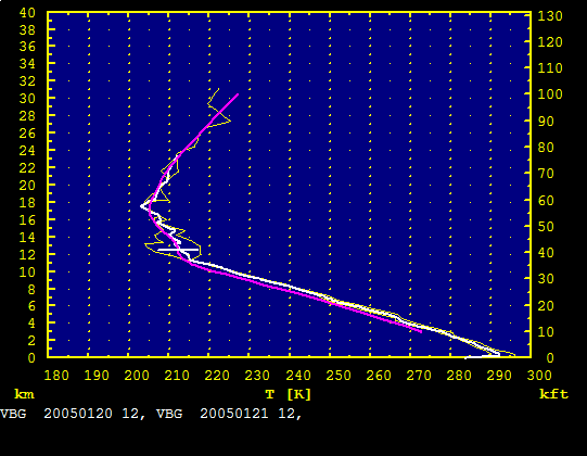
Figure 3. A RAOB/ATP comparison
from the January 20, 2005, PAVE fligth near Vandenburg AFB, CA.
Figure 3 shows a file named R34_20050120VBG.PNG from the PAVE
mission folder PNG subdirectory. The R34 at the beginning of the
filename indicates that this was the 34th comparison made for this
campaign, and is noteworthy in that there is substantial temperature
variability near the tropopause between these soundings (yellow) which
were 24 hours apart. (Note that if there were no missing or burst
soundings, they should always be <12 hours apart during
comparisons.) Nevertheless, the retrieved ATP (cyan) is in excellent
agreement with the temporally interpolated sounding (white). The
horizontal white bar is the average aircraft flight level at the time
of the flyby. The retrieved ATP does have a ~5 K cold bias in the
troposphere, but this was uncalibrated preliminary data. As mentioned
earlier, comparisons near the tropopause should be avoided if at all
possible. It is possible to filter these out later in the OATnavCOR
determination.

Figure 4. The RAOBcomparison.txt file imported
into an Excel spreadsheet.
As indicated above, the output from the comparison is written into a
text file named RAOBcomparison.txt
in the mission folder. This file is tab-delimited and readily imported
into an Excel spreadsheet as shown in Figure
4. Before proceeding further, find the RAOBcomparisonMISSION.xls
file from the last field campaign to use as a template. Using the Excel
File menu, Open it and then Save As in the current mission
folder, in our example, C:\MTP\Data\DC8\PAVE\.

Figure 5. The RAOBcomparisonPAVE.xls
window.
Copy the data in the RAOBcomparison.txt window and paste
it at the location of the yellow square in the
newly created RAOBcomparisonPAVE.xls
window H tab as shown
in Figure 5. Only a tiny
fraction of the data is visibile in this screenshot. We will show the
rest of it below.
The information on line 12 and below is as follows:
- Avg - the average difference between RAOB and ATP for each
comparison
- RMS - the standard deviation between RAOB and ATP for each
comparison
- Total - the population standard deviation between RAOB and ATP
for each comparison (the quadrature sum of the Avg and RMS)
- RAOB - launch site name
- Date - of comparison
- Distance - of aircraft from RAOB launch site
- Savg - average difference of two temporally interpolated
radiosondes
- Srms - RMS difference of two temporally interpolated radiosondes
- Frac - weight from 0 to 1 of first RAOB in temporal interpolation
- UTmtp - UT of comparison
- Zp - average pressure altitude at time of comparison
- Zt - average tropopause height at time of comparison
- Tn - average Tnav
- Tm - average Tmtp
- Tr - average Traob
- Tt - average Ttrop
- Tl - average layer temperature
- Tn -Tr : Tnav - Traob
- Tm - Tr : Tmtp - Traob
- Tn - Tl : Tnav - Tlayer
- Tm - Tl : Tmtp - Tlayer

Figure 6. The RAOBcomparisonPAVE.xls
window extending beyond Figure 5. and showing the temperature
comparisons between -10 and 0.5 km with respect to flight level. It
actually cover -10 to +10 km with respect to flight level if all could
be shown.
The information show in Figure 6 is the continuation to the right of
what was shown in Figure 5. When we first began doing these
comparisons, they were done in 500 m steps over a range of altitudes
appropriate for the aircraft. To do this, both the RAOBs and ATPs were
interpolated to a fixed grid of altitudes. The difficulty with this
approach is that it does not take account of the fact that the
comparisons are made with the aircraft possibly flying at different
altitudes. This would be fine if the performance was not pressure
altitude dependent, but it is. For the sake of argument, assume that
you have a fixed altitude grid on which you superimpose measurements
made when the plane is flying at FL330 and FL410. Clearly the retrieval
at 41, 000 feet is not going to be as good when flying at 33,000 feet,
as would be if the plane was actually at 41,000 feet. As a result the
performance is degraded the broader the range of altitudes at which
comparisons are made.
It is better to do the comparisons relative to flight level. The works
reasonably well as long as there are not huge optical depth
differences. For example, if a given flight had a boundary layer run
when most of the flight was at much higher cruise altitudes, then the
boundary layer run's performance should be handled separately. This is
what is now shown in Figure 6. We cover the range -10 km to +10 km in
0.5 km steps starting at -10 km in column W, reaching flight level in
column AQ, and +10 km in column BK (not visible). Rows 13 downward
simply report the difference between the RAOB and MTP temperature
profiles relative to flight level.
When the comparisons in Figure 5
and 6 were made, there were
originally 86 soundings available before additional editting criteria
were applied. In this case we simple deleted all soundings that had
temperature differences >3 K. This removed 9 of the soundings,
leaving 77. This number is entered in the cell F10, which is shown in
red to remind you to do it. If you don't do this, the accuracy
statistics will be incorrect.
The really interesting results appear in the top 10 rows of the
spreadsheet. Referring to Figure 5,
they show the following parameters starting with row 4:
- Average - the average
value for the column's parameter from row 13 to the bottom
- RMS - the rms value for
the column's parameter from row 13 to the bottom
- RMScorr - this used to
provide a performance correction for radiosonde sparce regions. It's
value was in cell F6, and it was removed in quadrature from the values
in row 5, the RMS
- Min - the minimum value
for the column's parameter from row 13 to the bottom.
- Max - the maximum value
for the column's parameter from row 13 to the bottom. The Min and Max
values are useful for checking that the editting criteria have been
met, such as a maximum temperature bias or distance from the tropopause
requirement.
- Total Error - This the
population RMS; or the
quadrature sum of Average and RMS
- SE - this is the standard
error on the Average, which is
RMS divided by the square
root of N-1, where N is the number of samples shown in cell F10.
The bottom line in doing all this of course is the value of OATnavCOR,
which can be found in Figure 5 cell I2 to be -0.77 K. When the data is
reprocessed using OATnavCOR = -0.77, and all the above steps repeated,
the result in cell I2 should be 0.0 K. This should be done to verify
that the sign of the correction is correct.

Figure 7.
Figure 8.
Previous | Next | Index |