MTP Pre-Campaign and Campaign Activities
MJ Mahoney
Last Revised: March 07, 2007
1. Measuring and Modelling the IF Bandpass
Introduction
Measuring and modelling of the IF bandpass should be performed before
and after every field campaign as it will affect the quality of
retrieval coefficient calculations. This is particularly important for
high altitude aircraft such as the ER-2, WB-57 and Geophysica because
the detailed line shapes become more important as pressure broadening
of the lines decreases, and they show more structure. RCcalc.exe, the program used to
calcualte retrieval coefficients, is the only program that uses the IF
bandpass shape. Like other aspects of the MTP data analysis, this
activity has evolved substantially over time. Historically, only the
DC-8 MTP used three frequency channels (CH1=55.51 GHz, CH2=55.65 GHz
and CH3=55.80 GHz), while the high-altitude aircraft used only the two
highest frequency channels because atmospheric transparency at high
elevation angles allowed little useful informaton to be measured in the
optically-thin lowest-frequency channel. For the past two years,
however, we have used three channels on all instruments. Although it is
true that the 55.51 GHz channel does not add useful information at high
elevation angles, it does provide useful information for the downward
looking elevation angles, and thus allows better tropopause solutions
on high-altitude aircraft flying above the tropopause.
Measurements
Early IF bandpass measurements involved tracing the voltage and/or
power bandpass shape off a spectrum analyser display onto quad paper,
or printing it if this was an option (generally involving an HPIB
interface). The trace would then be blown up using a zerox machine to
increase the size, and hence accuracy, of the plot. Pairs of points
representing the IF frequency and the response at this frequency would
then be manually entered into a spreadsheet. This was a very
tedious process. Current spectrum analyzers allow the spectrum to be
saved digitally in formats (such as comma separated variable (CSV))
that are easily imported into spreadsheets. Use the File | Open dialog box (showing All Files so non-xls files are
visible) to import a spectrum analyser CSV file into Excel; this will automatically open
a worksheet as shown in Figure 1.

Figure 1. CSV spectrum from HP
E4401B Spectrum Analyzer imported into an Excel spreadsheet.
Figure 1 shows the beginning of
a CSV file imported into an Excel
spreadsheet from measurements made on a HP E4401B spectrum analyzer of
the IF bandpass of the DC-8 MTP starting at 170 MHz (1.7E+08) in 75 kHz
steps. The tab was named CH1
to reflect the fact that this was a channel one spectrum measurement.
As indicated by the adjacent tab in the figure, spectra are also
imported for channel one with the noise diode on (CH1+ND), as well as the same
information for channels two and three as seen on adjacent tabs. In
addition, a CSV file is also imported (not shown) for the measurement
of the spectrum analyzer's noise baseline, which will be subtracted
from the spectrum measurements.

Figure 2. The All tab containing selected
information from the imported CSV file tabs.
Once all the CSV files have been imported, the Trace 1 information (see
column B of Figure 1) for each
is copied to a tab labelled All as
shown in Figure 2.

Figure 3. The AllNorm tab.
Finally, the normalized spectra are calculated on the AllNorm tab shown in Figure 3. The IF frequencies on the All tab are converted to MHz on the
AllNorm tab beginning at
column A line 24 (A24). Then each channel's spectrum has its baseline
removed in columns B, C and D. The normalized spectra are then
calculated as (CHn - Min)/(Max - Min)
in columns E, F and G, using the maximum (Max) and minimum (Min) values in Columns B, C and D to
perform the normalization. We will return to how the modelling is
performed below on this worksheet later.
Measured and Modelled IF Bandpasses for Existing MTPs

Figure 4. DC-8 MTP normalized
and modelled IF bandpass.
 normalized IF bandpass")
Figure 5. ER-2 sensor unit
number 1 (SU#1, or ER2S) MTP normalized and modelled IF bandpass.
 normalized and modelled IF bandpass")
Figure 6. ER-2 sensor unit
number 2 (SU#2, or ER2T) MTP normalized and modelled IF bandpass.
The normalized IF and modelled IF bandpasses for the existing three MTP
instruments are shown above in Figures
4-6 for the purpose of documenting this information and to
facilitate the discussion below. Also shown on the right-hand ordinate
axis are the upper and lower sideband molecular oxygen absorption
spectra.

Figure 7. The response change that results from introducing 1
dB of attenuation on the LO power level for the DC-8 MTP.
1) Frequency Dependence of IF Bandpass Shape
Until recently, we have made the reasonable assumption that the IF
bandpass for each frequency channel was the same. Indeed, given the
spectrum analyzer that we had been using, there was no discernable
difference between the three channels. Better equipment has shown that
not to be the case as a cursory examination of the traces labelled CH1, CH2 and CH3 in Figures 4-6 readily shows. The
largest differences are seen for ER-2 SU#2 shown in Figure 6. The exact reasons for
these differences are not known, but we suspect that it has to do with
LO power level differences and small frequency dependent impedance
mismatches. Measurements have been made with 1 dB less LO power on the
DC-8 MTP, and the bandpass changes by up to 4% (see Figure 7).

Figure 8. Molecular oxygen
absorption spectrum observed by the MTP.
2) Matching Bandpass Shape to Upper and Lower Sidebands
All of the existing MTPs use double-sideband (DSB), rather than
single-sideband (SSB), receivers. While this doubles the signal
detected per unit time, which improves the signal-to-noise ratio, it
introduces other complications. This is particularly important for the
high-altitude instruments where details of the lines shape become more
important because of the reduced pressure broadening. In particular, as
shown by the 20 km absorption spectrum in Figure 8 (red trace), the line
absorption strength in the two sidebands is generally different for any
pair of selected lines (which means that the effective "look" distances
are different), and the lines pairs are not all separated by the same
frequency interval (which means that the position of the lines within
the IF bandpass will be different). It really makes more sense to
me at to use single sideband receivers on high-altitude platforms, but
we have not been able to pursue this option.
In addition to the IF bandpass measurements shown in Figures 4-6, the upper sideband
(USB) and lower sideband (LSB) oxygen absorption spectra are also
shown. These are needed to match the IF bandpass to the upper and lower
sidebands of the MTP. This is more easily done at DC-8 altitudes
(<12.5 km) than at ER-2 altitudes (20 km) because the stronger
pressure broadening of the oxygen absorption lines results in much less
structure across the IF bandpass. Note in Figure 7 that on the ground
(green trace) the pressure broadening is so strong that the 40 spectral
lines making up the molecular oxygen absorption spectrum show little
structure. This point is also made by comparing the USB/LSB lines in Figure 5 for the DC-8 to the lines
for the ER-2 (and other high altitude aircraft) shown in Figure 5 and 6. There are a number of issues
which must be addressed, the first being that the two sidebands don't
have the same shape or absorption. If the bandpass had a square
response, the LO frequency would be adjusted so that the lines
representing the two sidebands had their peak at the center of the
bandpass. This can't always be done exactly because the lines in the
three channels (which share the same IF) aren't separated by the same
frequency interval. To further complicate matters, the IF bandpass is
not always flat, as is apparent in Figure
5 for MTP SU#1 which has a pronounced slope. That is why the LO
was chosen so that the CH3 USB peak response (pink) was located where
the IF bandpass was reduced. However, the same LO frequencies are not
optimum for ER-2 SU#2 because it has a much flatter response. When this
unit was built, we blindly used the same LO frequencies because the
"corporate memory" and how the LO frequencies were chosen has been
forgotten, and wasn't documented anywhere. Later on this page we will
discuss a program (Bandpass.vbp)
which has been written to optimize the LO frequencies. It should also
be noted by comparing the DC-8 m
Optimizing the LO Frequencies
The import process is very straightforward, as is shown in Figures 1
and 2.
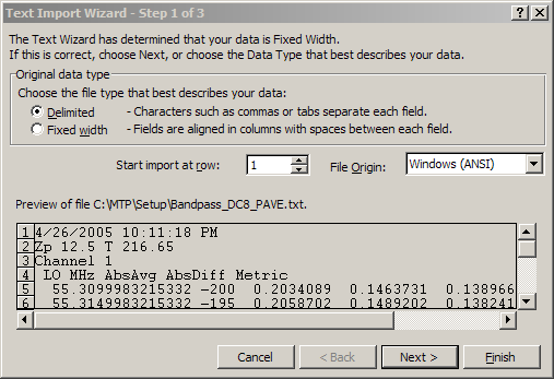
Figure 1. When a CSV file is selected using the File|Open menu option,
it is automatically recognized and imported as shown in the figure
above. Select the options as shown.

Figure 2. In the next step, select the Tab and Space Delimiters and
click the Next button to complete the import process.

Previous | Next | Index |