
 SHEBA ISFF Flux-PAM
Project Report
SHEBA ISFF Flux-PAM
Project Report
SHEBA ISFF Flux-PAM
Project Report
SHEBA ISFF Flux-PAM
Project Report
NCAR Flux-PAM stations used two different types of sonic anemometers
over the duration of the SHEBA project.
In October 1997, the PAM stations were instrumented with
Gill R2 Solent sonic anemometers.
In order to mitigate riming problems, three of these were replaced with
Applied Technologies (ATI) sonic anemometers, beginning at the end of
February 1998.
A second measure to reduce the riming was the addition of
electrical heaters on the sonic transducers,
beginning in early January 1998.
The use of ATI sonic anemometers and transducer heaters,
along with the onset of spring, significantly reduced the loss of
turbulence data due to riming after February 1998.
9.2 Laboratory testing of R2 Solent sonic anemometers
During planning for the SHEBA project, recognition of the potential for riming of the sonic anemometers led to the choice of the Gill Instruments R2 Solent for use on the Flux-PAM stations. This choice was based on their low power requirements, favorable NCAR experience with their operation during rainfall, Gill Instrument's published specification that they would operate down to -40 °C and with a coating of ice up to 2-3 mm thick, and a report from Andy Black at the University of British Columbia of successful operation down to -35 °C ("except when the coating of hoar frost or snow got too thick").
Since NCAR has only one Gill sonic anemometer, five additional R2 Solents were borrowed from Chris Fairall at NOAA Environmental Technology Laboratory, Carl Friehe at the University of California at Irvine, and Jim Edson at Woods Hole Oceanographic Institute. During the summer of 1997 these sonics were tested in the NCAR Sensor Calibration Laboratory for low-temperature operation. Tests were conducted in a chamber that was just large enough for a single Solent to fit diagonally between opposite corners, with the measurement array within a few inches of two of the chamber walls and the top of the chamber. The chamber temperature was typically ramped from 25 °C to -45 °C in a 12-hour period, held at -45 °C for one hour or more, and then ramped back up to 25 °C over another 12 hours. The sonic data were sampled at 21 Hz, and statistics (means, variances, etc.) were calculated in 5-minute blocks.
The principle statistics used to quantify sonic performance were the 5-minute variances of the three orthogonal wind components and sonic temperature. A more detailed look at a limited subset of the data used 10-minute calculations of the power spectra and cospectra. The performance of four of the sonics was acceptable down to -35 °C and somewhat degraded at lower temperatures. The velocity variances gradually increased with decreasing temperature, as an example from 0.05-0.10 m²/s² at 25 °C to 0.05-0.13 m²/s² at -30 °C. Below -30 °C the variances increased more rapidly, typically to 0.08-0.2 m²/s² at -40 °C. Below -30 °C there was evident noise contamination of the power spectra in the inertial subrange, particularly for sonic temperature. The contamination generally increased with decreasing temperature. Two of the sonics were not acceptable below -30 °C to -35 °C. Below those temperatures the variances increased very rapidly to levels of 10-100 m²/s² or more.
There was a noticeable and repeatable modulation of the variance amplitudes through the tested temperature range, with a period of 6-7 °C. This corresponds to one period of the 180 kHz sonic pulse. Angus Raby of Gill Instruments suspects that this is caused by reflections of the pulses from the walls of the chamber. This modulation was present for all R2 Solents, but was not present for an R3 Solent or a Campbell CSAT3 sonic. However it was possible to locate the Campbell sonic more centrally in the chamber (further from the walls), and it operates at 400 kHz, which would cause more atmospheric attenuation of the reflected signals. Angus also suggested that the more sophisticated 32-bit signal processing of the R3 and Campbell sonics is better able to discriminate against reflected signals. At the suggestion of Angus, it was tried (unsuccessfully) to attenuate the reflections with a thin layer of felt lining in the chamber. Thus the modulation was not an artifact of the chamber ventilation system, but it was not shown conclusively that it was caused by reflections from the chamber walls.
One of the poor-performance R2 Solents was sent to Gill Instruments for testing and it appears that they were able to identify one cause of increased variance below -30 °C. An ultrasonic transducer continues to ring for a time after it has transmitted a pulse. Since a transducer serves alternately as transmitter and receiver, at low temperatures (below -30 °C) there is sometimes enough signal left from when the transducer last transmitted to prematurely trigger the next detection of a received pulse. Angus Raby was able to reduce these false triggers by decreasing the sensitivity of the receiver, but this is not the ideal solution for two reasons:
Nevertheless, this modification was implemented on all R2 Solent sonics used on the SHEBA Flux-PAM stations.
During testing, Angus Raby also discovered that transducer ringing
got worse as they started to ice up.
A layer of ice 0.5 mm thick was found to cause false triggering of the
receiver at low temperatures when the true receive signal is reduced.
This behavior is not consistent with Gill's published performance
specifications of acceptable operation with a coating of 2-3 mm of ice.
9.3 Field performance of R2 Solent sonic anemometers
The field performance of the R2 Solent sonics during the fall and winter of 1997 was quite disappointing.
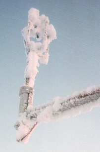
|
| E. Andreas, October 25, 1997 |
Second, the Solent sonic performance appeared to be very sensitive to riming, as suggested by Angus Raby's tests. When cleaning frost off the Solent sonics, it was often inadequate to simply brush off the feathery frost, and sometimes required tediously melting a thin residual base coat of ice to restore acceptable performance (often at the expense of cold fingers). In contrast, the ATI sonics used on the Atmospheric Surface Flux Group meteorological tower in the main camp were not nearly as sensitive to riming and could often be restored to operation simply by brushing off the feathery frost.
Riming of the Solent sonics was accompanied by a noticeable
degradation of the quality of the wind and temperature data,
characterized in particular by increasingly noisy data.
The Solent outputs data at a rate of 21 Hz, and each datum is
nominally the average over eight acoustic pulses.
However, the Solent firmware performs an internal quality check on
each of the pulses and averages only acceptable pulses into
the output data, reporting an invalid wind value (-100 m/s) if
an inadequate number of pulses is acceptable.
(Note that because the Solent sonic array is non-orthogonal,
unacceptable pulses on any one transducer path cause all of the
outputs to be reported as invalid.)
The valid wind samples are averaged by the EVE data system, which
also calculates the percentage of valid samples in each 5 minute set
of wind and turbulence statistics as the data variable
samples.sonic.
Riming of the Solent sonics is detectable as a decrease in
samples.sonic below 100%, and this provides a somewhat objective
measure of Solent data quality.
There is not a precise threshold value of samples.sonic that unambiguously
separates good data from bad, but it appears that a reasonable working value
is on the order of 99%.
If it is desired to err on the side of filtering out good data in the
quest to maximize the elimination of erroneous data, then 99.9% is not
too large a value for this threshold.
9.3.2 Path curvature correction
The R2 Solent sonic anemometer outputs three orthogonal wind components
(u,v,w) plus the speed of sound, c.
The EVE data system then calculates sonic virtual temperature
tc from the speed of sound and wind component data,
including a "path curvature" correction,
tc = a(c2 + vn2)
where vn is the velocity component normal to the sonic path used to measure the speed of sound and a = 2.48e-3 °K-s²/m². Prior to June 21, 1998, EVE incorrectly used the formula
vn2 = v2 + (u2 + w2)/2
whereas the proper formula is
vn2 = v2 + (u + w)2/2
where u,v,w are the velocity components in an orthogonal coordinate system aligned with the sonic measurement array. The corrections to the five-minute-averaged first and second moments of the Solent data output by EVE are
<tc> = <tE> + a(<u><w> + <u'w'>)
<u'tc'> = <u'tE'> + a(<u><u'w'> + <w><u'u'>)
<v'tc'> = <v'tE'> + a(<u><v'w'> + <w><u'v'>)
<w'tc'> = <w'tE'> + a(<u><w'w'> + <w><u'w'>)
<tc'2> = <tE'2> + 2a(<u><w'TE'> + <w><u'TE'>) +
a2(<u>2<w'w'> + 2<u><w><u'w'> + <w>2<u'u'>)
where <x> denotes a five-minute average of the
variable x and tE is the
sonic virtual temperature as incorrectly calculated by EVE.
These corrections have been applied during data post-processing at
NCAR.
9.4 Sonic heaters
During November and December, heaters were developed at NCAR that could be attached to the sonic transducers in order to melt the rime ice.
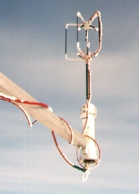
|
| E. Andreas, May 17, 1998 |
Initially, the microprocessor was programmed to turn on the heaters
at regular intervals, for example 5 minutes per 2 hours.
However, this proved to be difficult to sustain because regular use
of the heaters drained the station batteries.
A better solution was implemented on February 20 when software was
installed on the shipboard base computer to turn on the heaters via
the RF modems only when the station battery voltage exceeded 12 V
and the sonic firmware reported a deterioration in
sonic performance (less than 99.5% of the sonic samples acceptable).
The data parameter heater, recorded for each station,
corresponds to the fraction of time during each 5-minute data sample
when a sonic heater is turned on.
9.5 Replacement of R2 Solents with ATI sonic anemometers
In 1997, Applied Technologies began producing a new version of their sonic anemometer that reduced the power requirement to less
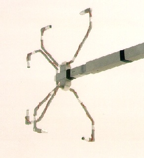
|
| E. Andreas, May 15, 1998 |
The ATI sonic outputs data at a rate of 10 Hz and each datum
is nominally the average over 20 acoustic pulses.
Unacceptable pulses are again detected by internal quality checks
and excluded from the averages.
In contrast to the Solent, however, the number of acceptable pulses
along each transducer path is included in the ATI output data and
archived in the 5-minute PAM data as
usamples, vsamples and wsamples.
Since the ATI array is orthogonal, a problem with one transducer
path does not invalidate data from the other component paths.
For the ATI, the variable samples.sonic was initially
equivalent to wsamples, but around the end of April
(April 25 for stations 1 and 2, May 1 for station 3)
samples.sonic was changed to be calculated by summing
the number of acceptable pulses along all three paths
and dividing by the total number of pulses.
9.6 Sonic anemometer heights
The heights of the sonic anemometers were measured when the Flux-PAM stations were deployed in October 1997 and then during many service visits from April until September 1998. The Solent sonic arrays were nominally 58 cm above the boom and the ATI sonic arrays were at essentially the same height as the boom. The Solent sonics were on the order of 3.5 m above the surface, while the ATI sonic heights varied (due to surface ablation) between 2.25 m and 3.25 m. The detailed sonic height measurements are tabulated below, based on entries in the PAM logbook.
| Station 1 | Station 2 | Station 3 | Station 4 | ||||
|---|---|---|---|---|---|---|---|
| Date | Ht(m) | Date | Ht(m) | Date | Ht(m) | Date | Ht(m) |
| 97 10 15 | 3.46 | 97 10 15 | 3.46 | 97 10 15 | 3.45 | 97 10 23 | 3.48 |
| 98 04 11 | 2.26 | 98 04 11 | 2.82 | 98 04 22 | 2.46 | 98 04 11 | 3.33 |
| 98 04 17 | 2.26 | 98 04 16 | 3.45 | 98 05 15 | 2.34 | 98 04 20 | 3.20 |
| 98 05 21 | 2.22 | 98 05 16 | 2.87 | 98 06 18 | 2.63 | 98 05 16 | 3.42 |
| 98 06 12 | 2.39 | 98 06 12 | 3.02 | 98 06 29 | 2.68 | 98 06 08 | 3.47 |
| 98 06 22 | 2.51 | 98 06 23 | 3.03 | 98 07 09 | 2.69 | 98 06 13 | 3.48 |
| 98 07 06 | 2.77 | 98 07 07 | 3.12 | 98 07 30 | 2.97 | 98 07 29 | 3.51 |
| 98 07 21 | 2.87 | 98 07 23 | 3.24 | 98 08 10 | 2.97 | 98 08 26 | 3.53 |
| 98 08 03 | 2.92 | 98 07 30 | 3.23 | 98 08 24 | 2.93 | 98 09 08 | 3.51 |
| 98 08 29 | 3.57 | 98 08 26 | 3.28 | 98 09 20 | 2.92 | 98 09 20 | 3.50 |
| 98 09 16 | 3.48 | 98 09 16 | 3.26 | 98 09 30 | 3.52 | ||
| 98 09 30 | 3.31 | ||||||
Determination of absolute wind directions from the sonic anemometer data requires knowing the horizontal orientation or azimuth of their u and v measurement axes. The wind direction relative to true North is calculated as atan(-u,-v) + Vazimuth, that is, a positive v wind component is blowing from the direction Vazimuth + 180°. The alignment of the v axis, Vazimuth, is calculated as
Vazimuth = compass + declination + orientation
Here compass is the data provided by an electronic magnetometer compass mounted on the PAM mast, declination is provided by the GPS receiver at each station, and orientation is the angle between the sonic positive v axis and the North axis of the electronic compass. The overall uncertainty of the compass data is estimated to be ±3°, and the uncertainty of the orientation correction is at times as large as perhaps ±5°, particularly for the Solent sonics. A check of long-term-average wind directions calculated for the four stations shows them generally to be equal within at least ±8° and often to agree within ±3° or less.
The electronic compass was mounted on top of the hygrothermometer and oriented with its North axis nominally 90° counterclockwise from the boom on which the sonic was mounted. Several problems occurred with the electronic compass data during the project. Prior to October 20, 1997, a software bug caused the compass data to be lost so that any absolute wind directions prior to that date use the compass reading on October 20. Initially, there was also a problem in the hygrothermometer which caused spiking on the compass data once every 3-10 hours. This was fixed at Florida on October 23, Atlanta on October 24, Baltimore on October 25, and at Cleveland on October 26. As noted in Section 6, these spikes were removed during data post-processing. Spiking was also caused by operation of the sonic heaters. These spikes have been flagged as missing data during data post-processing and replaced with interpolated data during calculation of Vazimuth. Swapping the hygrothermometer and/or the compass at a station often caused a step change of 1° to 3° in the compass reading, but the exact cause of this change or an objective correction procedure is not immediately obvious. Finally, operation of the beacon light reduced the compass readings at that station by 1°-4° while the beacon was turned on. The compass data have been nominally adjusted during post-project analysis for the offset caused by beacon operation.
The compass data at Florida are obviously in error for a 27-hour period on September 18-19, 1998. These data have been replaced with interpolated values. The compass data at Maui is questionable and often missing from roughly August 1 to September 4, 1998. Logbook entry 666 notes improving the operation of this compass on September 2 by draining water out of it! However, it is not immediately obvious which data are good and which are bad during most of this time period. The only corrective action for the Maui compass data has been to replace intermittent data from August 23 to September 2 with interpolated data. Hand-held compass readings were taken during station visits in the spring and summer. These were generally consistent with the electronic compass readings, but their accuracy was judged to be insufficient to eliminate residual uncertainties on the order of ±3° in the true orientation of the compass.
The declination is determined from an internal table in the GPS receiver as a function of the measured latitude and longitude. For most of the project, the declinations of the four Flux-PAM stations were within 0.1°-0.2° of each other; but in September 1998, Baltimore drifted further away from the other stations, and its declination approached a value 0.5° greater than the others. However, in order to provide a robust value of the declination for calculation of sonic azimuth and because the declinations of the four stations were equal to each other within the accuracy of the compass and orientation data, the median value of the declination values from all reporting stations is used to calculate sonic azimuth at each station.
The orientation is the angle between the orientations of
the positive v axis of the sonic
and the North axis of the electronic compass.
For the ATI sonic, with its u axis parallel to the sonic boom and
positive for winds blowing toward the mast,
this angle is nominally equal to 180°.
The R2 Solent sonics have a North arrow inscribed on the top,
which is oriented 30° clockwise from the negative u axis
of the data output by the anemometer.
By convention, NCAR orients this North arrow to be pointed away from
the tower and parallel to the boom on which the sonic is mounted,
so that the orientation angle is nominally 150°.
For the asymmetrical (R2A) Solent anemometer, this orients the
least-obstructed portion of the sonic array in the direction
directly away from the tower.
On occasion, however, a Solent sonic was mounted for a period
of time with the North arrow not pointing along the boom.
To the best of our ability, this has been accounted for in the sonic
orientation,
based on field notes in the PAM electronic logbook.
Again, the hand-held compass readings were judged insufficient to
eliminate residual orientation uncertainties of ±5°.
9.8 Post-project calculation of sonic tilt
Tilt of a sonic anemometer from true vertical can introduce errors in the measured sensible heat and momentum fluxes. The tilt error in u* or in a scalar flux is on the order of 5% per degree of tilt in the vertical plane aligned with the mean wind direction. Consequently, it is often necessary to rotate the coordinates of three-dimensional sonic wind data to correct for this tilt. NCAR estimates the sonic tilt angles from the archived wind data using the planar fit technique described in Wilczak, Oncley, and Stage, 2001, `Sonic anemometer tilt correction algorithms', Boundary Layer Meteor., 99, pp. 127-150. Briefly, this technique assumes that the time-averaged wind field is confined to a plane surface, nominally parallel to the ground. It is assumed that the fluxes of interest are those normal to this wind-field plane and thus the vertical velocity axis is re-oriented normal to that plane. The orientation of the wind-field plane relative to the measurement axes of the sonic anemometer is determined by a least-squares fit of the wind data to the equation
w = a + bu + cv
where u, v, w are the 5-minute-averaged horizontal and vertical wind components measured by the sonic anemometer. The fitted coefficients correspond to
vertical velocity offset = a
sonic lean angle = atan((b2 + c2)½)
azimuth of sonic lean (relative to u axis) = atan(c/b)
Confidence in the fit to this model requires data with as wide a range of wind directions as possible; in practice, 90° or greater. Thus confidence can best be achieved with data extending over many hours or days. If the data are available, this requirement is acceptable because the sonic tilt angles are expected to be unchanged unless the sonic anemometer is moved (or the surrounding surface itself changes!). Thus the tilt angles are calculated for periods delimited by known physical changes in the sonic orientation, e.g. re-leveling the mast or swapping the sonic anemometer.
The wind data used to calculate the SHEBA tilt coefficients were edited using several criteria to increase the reliability of the least-squares fit. The analysis used data for each five minute period only when 99.9% of the samples were judged acceptable by the sonic firmware and when the transducer heaters were not operated during the period. Wind directions within ±45° of the mast were also eliminated from the analysis, as were wind speeds less than 1 m/s. Finally, the fraction of data acceptable to a spike-detection routine running on EVE was required to exceed 99% for each 5 minute period.
The vertical velocity offsets a derived from the least-squares planar fits were generally found to be higher for the R2 Solents than for the ATI sonics, 5-15 cm/sec versus 1-2 cm/sec. However, plots of w versus wind speed for each period suggest that the true w offset is quite small for both the Solent and ATI sonics. For low-noise data with a wide range of wind directions, these plots are a well-defined wedge which is symmetrical about the w=0 axis and points toward speed=0. For example, see Fig. 9.8.1a for a plot of the data from Station 3 beginning on April 22. Fig. 9.8.1b shows the corresponding plot of the planar fit for that period. (See below for a discussion of the planar fit plots.) For a period with a narrow range of wind directions there may only be data either above or below the w axis, Figs. 9.8.2a and 9.8.2b, and for the Solent sonics there is often a great deal of scatter in these plots, Figs. 9.8.3a and 9.8.3b. Nevertheless in almost every case, there appears to be no significant displacement of the line of symmetry from the w axis, as would be caused by a w offset. It is concluded that the large w offsets calculated by the least-squares fit to the Solent data are simply an artifact of noisy data associated with heavy riming, and the least-square planar fits were recomputed assuming a=0. (The only exception is the Atlanta sonic for the period beginning on July 6, 1998. For that period there is a definite offset of -10 cm/s.) The plots of w versus wind speed also provided an additional editing parameter for the planar fits, a maximum allowable vertical elevation angle which was individually specified for each analysis period.
The calculated values of the sonic lean angle and the lean azimuth are tabulated below for the four Flux-PAM stations. Each entry shows the date and time at the beginning of the period for which the entry is applicable, as well as the specific sonic used during the period. Also tabulated are the rms residuals from the least-squares fit. The tables are followed by brief discussions of the analysis.
The tilt fits to the ATI data are generally much better than the fits to the R2 Solent data. This is quantitatively reflected in the rms residuals, 2-4 cm/sec for the ATI data versus 10-20 cm/s for the Solents. Presumably this is because a greater sensitivity to riming causes the Solent data to be much noisier than the ATI data, even after the editing described above. However, an additional contributing factor might be that heavy riming of the support structure of the more-enclosed Solent sonic array (only the transducers are heated) may at times have significantly distorted the flow through the array. The lean angles are also generally higher for the Solents, 1°-4° versus 0.5°-2° for the ATIs. This could reflect the fact that the Solent array is more difficult to mount precisely vertical than the ATI, be caused by flow distortion within the array, or again simply be an artifact of the noisy Solent data. The sonic wind data and the tilt fits can be displayed as plots of wind elevation angle, atan((w-a)/(u2+v2)½), versus wind direction (azimuth) relative to the sonic u axis. These plots can be accessed from the links in the first column of the tables. In this representation, the least-squares planar fit is a sinusoidal curve with a period equal to 360° of wind direction. The tables include a signal-to-noise ratio in this representation, equal to the the calculated lean angle divided by the rms deviations of the wind elevation angles from the fitted sinusoidal curve. Finally, the tables include a comment on the quality of the fit, based on a subjective assessment of these plots. Since some of the periods had data with a limited range of wind directions (sparse fit) or very noisy data (poor fit), the calculated tilt parameters were at time not used to reorient the sonic data. This subjective decision, based on the individual plots, is indicated in the last column of the tables. In general the acceptable fits have a S/N > 1 and the unacceptable fits have S/N < 1, but there are inevitably a few exceptions. Note that the ATIs at times had lean angles on the order of 0.5° accompanied by a small signal-to-noise ratio. Although the corresponding lean and azimuth angles have not been used to reorient the sonic data, the consequences are minimal because the lean angles are small.
| Date | Time | Sonic | Lean | Azimuth | RMS | S/N | Comment | Rotated |
|---|---|---|---|---|---|---|---|---|
| GMT | (deg) | (deg) | cm/s | |||||
| 97 10 11 | 00:00 | R2 0112 | 3.5 | -179.8 | 4 | 3.9 | sparse | yes |
| 97 10 15 | 22:00 | R2 0112 | 1.4 | 167.8 | 19 | 0.8 | poor | no |
| 98 01 15 | 20:00 | R2A 0087 | 1.7 | 72.5 | 34 | 0.3 | poor | note 1 |
| 98 02 20 | 22:00 | R2A 0087 | 2.3 | 87.8 | 13 | 1.5 | fair | yes |
| 98 03 20 | 20:00 | ATI 980202 | 1.1 | -143.7 | 4 | 2.8 | good | yes |
| 98 04 18 | 20:30 | ATI 980202 | 0.5 | -131.1 | 3 | 1.3 | fair | no |
| 98 05 19 | 00:00 | ATI 980202 | 0.5 | 139.0 | 3 | 1.0 | fair | no |
| 98 06 11 | 00:00 | ATI 980202 | 1.0 | 144.8 | 3 | 2.0 | fair | yes |
| 98 07 06 | 20:00 | ATI 980202 | 0.1 | -104.6 | 3 | 0.1 | fair | no |
| 98 07 27 | 00:00 | ATI 980202 | 0.5 | -68.1 | 4 | 0.6 | fair | no |
| 98 08 24 | 21:00 | R2A 0067 | 1.8 | 84.5 | 6 | 1.8 | sparse | no |
| 98 08 27 | 00:30 | R2A 0067 | 4.3 | -150.1 | 12 | 1.7 | sparse | no |
| 98 08 29 | 22:00 | R2A 0067 | 1.2 | 168.1 | 14 | 0.5 | fair | no |
Note 1: Used lean and azimuth angles from following period
Because of icing, good R2 0112 data are very scarce from October 1997 to January 15, but there is a fair distribution of wind directions. The data are split on October 15 when the sonic was reoriented in its mount by 90°. The data for Solent R2A 0087 with heaters are divided into two separate periods by the introduction of base-software heater control on February 20. Good data are again moderately scarce before February 20, because the heaters were used only sparingly to conserve battery power. The data after February 20 are moderately complete and have a good range of wind directions. However, because of the large data scatter, it is not clear whether the Solent data fit the model used to find the sonic orientation. There is no known cause for the change in parameters on February 20, except possibly flow distortion due to excessive riming prior to February 20. Thus we have used the lean and azimuth angles calculated for the period beginning on February 20 to rotate the R2A 0087 data for the preceding period.
As noted previously, the ATI data are significantly less noisy than the Solent data. The ATI 980202 data have been divided into six distinct periods. The first period ends on April 18 when the tripod was releveled. The data from April 18 to July 6 were divided into three periods in an attempt to capture the presumed change in level of the tripod during the melting season beginning in mid-May. (There was noticeable, systematic change in the radiometer electronic levels during this period.) Then in early July there was an unexplained (by the logbook) change in the character of the vertical velocity, in particular a change in the mean vertical velocity. There was a second, less prominent, change in character around July 27.
The Atlanta ATI v axis failed in mid-August and was replaced by Solent R2A 0067 on August 24. The Solent installation was modified on August 27 and 29. Again the Solent data have much more scatter than the ATI data, so the results should be judged less reliable.
| Date | Time | Sonic | Lean | Azimuth | RMS | S/N | Comment | Rotated |
|---|---|---|---|---|---|---|---|---|
| GMT | (deg) | (deg) | cm/s | |||||
| 97 10 14 | 00:00 | R2A 0067 | 1.1 | 125.5 | 12 | 1.0 | fair | no |
| 98 04 06 | 19:00 | ATI 980303 | 1.0 | -132.8 | 2 | 3.3 | sparse | yes |
| 98 04 18 | 04:00 | R2A 0123 | 3.9 | -117.9 | 10 | 3.3 | sparse | yes |
| 98 04 22 | 18:15 | ATI 980302 | 0.4 | 175.5 | 6 | 0.6 | poor | no |
| 98 06 11 | 00:00 | ATI 980302 | 1.7 | -144.1 | 3 | 3.4 | good | yes |
| 98 07 12 | 00:00 | ATI 980302 | 1.8 | -109.7 | 4 | 2.3 | good | yes |
| 98 08 20 | 00:00 | ATI 980302 | 1.9 | -160.4 | 3 | 3.8 | good | yes |
Because of icing, good data are very scarce for Cleveland from October 1997 to February 6, 1998, when Cleveland was damaged by a closing lead, but there is a fair distribution of wind directions.
Station 2 was used to test ATI 980303 from April 6-13, and data are quite sparse for this period. Station 2 was resurrected at the Seattle site on April 16, but the Solent sonic was only there for 5 days before being replaced by an ATI on April 22. The data for April 18-22 are very sparse. The data for ATI 980302 at Seattle (April 22 - June 10) have a notable signature for wind from the ENE, characterized by a full cycle of the elevation angle from 0° to +2° to 0° to -2° and back to 0° over a wind direction range of about 35°. This may well have been caused by a pressure ridge only about 50m to the north.
On June 11, station 2 was moved to the Maui site. It might be noted that the ENE wind elevation signature from Seattle does not appear at Maui, supporting the assumption that it was caused by the local topography. The succeeding data have been divided into three periods that appear to be internally consistent in the tilt parameters. The derived lean angle of almost 2° is not consistent with a logbook note on August 30 stating that the sonic was level within 0.5°.
| Date | Time | Sonic | Lean | Azimuth | RMS | S/N | Comment | Rotated |
|---|---|---|---|---|---|---|---|---|
| GMT | (deg) | (deg) | cm/s | |||||
| 97 10 12 | 00:00 | R2A 0087 | 1.3 | -4.8 | 3 | 1.4 | sparse | no |
| 97 10 15 | 19:00 | R2A 0087 | 1.5 | 18.7 | 11 | 1.4 | fair | yes |
| 98 01 13 | 20:30 | R2A 0123 | 1.3 | 60.9 | 15 | 1.0 | poor | Note 1 |
| 98 02 20 | 22:00 | R2A 0123 | 1.5 | -97.5 | 14 | 0.8 | fair | yes |
| 98 04 15 | 02:00 | ATI 980303 | 1.5 | 168.2 | 3 | 3.8 | good | yes |
| 98 04 22 | 03:00 | ATI 980303 | 1.6 | 150.0 | 3 | 4.0 | good | yes |
| 98 06 24 | 00:00 | ATI 980303 | 0.9 | 144.0 | 3 | 1.5 | good | yes |
| 98 07 03 | 00:00 | ATI 980303 | 0.8 | -8.1 | 3 | 1.3 | fair | yes |
| 98 07 12 | 00:00 | ATI 980303 | 2.2 | 10.1 | 2 | 4.4 | good | yes |
| 98 07 21 | 00:00 | ATI 980303 | 1.2 | 170.6 | 2 | 3.0 | sparse | yes |
| 98 07 31 | 00:00 | ATI 980303 | 0.4 | 44.4 | 3 | 1.0 | good | yes |
Note 1: Used lean and azimuth angles from following period
Because of icing, good data are very scarce for Baltimore from October 1997 to January 13. The data are split on October 15 when the sonic was reoriented in its mount by 90°. The distribution of wind directions is very limited, so the derived tilt parameters are somewhat speculative. Even the addition of heaters did not improve the data recovery until the base heater control software was installed on February 20. Again, the lean and azimuth angles for February 20 - April 14 were used to rotate the R2A 0123 data for the January 13 - February 20 period. Although the February - April data are quite scattered, there is a good distribution of wind directions.
The data for ATI 980303 from April to September are divided into seven periods based on apparent changes in the tilt parameters. In particular, extensive melting of the surface and possible settling of the tripod appears to have occurred during the period from June 24 - July 31. The tripod was releveled on April 22, July 20 and July 30.
| Date | Time | Sonic | Lean | Azimuth | RMS | S/N | Comment | Rotated |
|---|---|---|---|---|---|---|---|---|
| GMT | (deg) | (deg) | cm/s | |||||
| 97 10 23 | 00:00 | R2A 0123 | 0.6 | 52.8 | 12 | 0.5 | poor | no |
| 98 01 13 | 20:30 | R2A 0087 | 11.7 | 83.6 | 7 | 7.3 | sparse | yes |
| 98 01 18 | 04:45 | R2 0112 | 4.1 | 121.4 | 16 | 1.8 | fair | yes |
| 98 02 26 | 22:00 | ATI 980202 | 0.8 | 155.3 | 3 | 1.3 | good | yes |
| 98 03 20 | 20:00 | R2A 0087 | 4.1 | 100.9 | 13 | 2.6 | fair | yes |
| 98 04 02 | 00:00 | R2A 0087 | 1.4 | 148.3 | 10 | 1.1 | fair | no |
| 98 04 20 | 23:30 | R2A 0087 | 1.4 | 86.3 | 12 | 0.9 | fair | no |
| 98 06 05 | 23:30 | R2A 0087 | 3.1 | 153.6 | 11 | 1.9 | good | yes |
| 98 07 30 | 04:30 | R2A 0087 | 1.5 | -172.8 | 16 | 0.8 | fair | yes |
There is a large amount of scatter in the wind data for the R2A 0123 sonic from October to early January, and consequently the tilt fit is poor. Fortunately, the indicated lean is only 0.6°. During January and February there were several changes of anemometers at Florida associated with implementation of the heaters and introduction of the first ATI sonic. R2A 0087 was used for only a few days in January, and consequently the data available for the tilt fit are quite sparse. Although the direction range is limited, the fit looks good, lending some plausibility to the large derived lean angle (11.7°). The data for R2 0112 again contain a large amount of scatter, but the wind direction range is good and the fit appears plausible. The fit for ATI 980202 is quite good.
The data for R2A 0087 from March 20 until October are divided into five periods by four moves of the Florida station during that time. There is a fair amount of scatter in the data, and consequently the fits are at times somewhat questionable. In particular, the period April 2-20 has sparse data and the period April 20 - June 5 also appears questionable. On the other hand, the fit for June 5 - July 30 is one of the best achieved with an R2 Solent sonic during SHEBA.
| Table of Contents | Previous | Top | Next |