If you reached this page from a search engine, click here to see the full report, with frames.
The first phase of that project is described in a separate document.
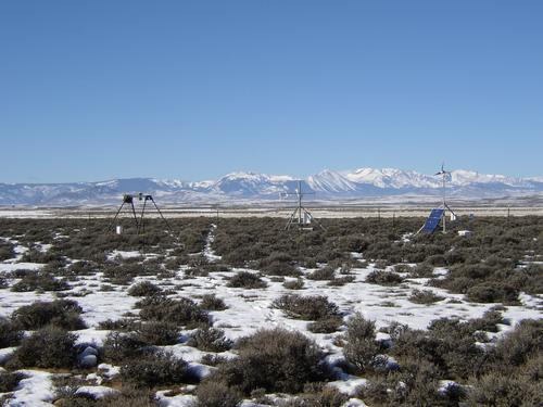
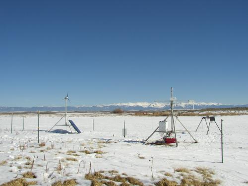
This document is a standard product of NCAR/ATD/RTF which gives an overview of the measurements taken using the Integrated Surface Flux Facility (ISFF) and conditions during the FLOSSII field experiment.
FLOSSII will operate in conjunction with the NASA Cold Land Processes Field Experiment (CLPX).
The Refuge also has supplied us with an aerial photo of the area around our site from a few years ago, which I've anotated with approximate locations of the FLOSS and FLOSSII sites.
We've produced a map; using Topo of the site, with tower locations for FLOSS01 and FLOSSII indicated with red dots. Note that the labels are to the NE of the corresponding dot -- not necessarily the closest.
I have written a set of driving directions for the convenience of the many visitors we expect to see! Also, see my contact list for our phone numbers, etc.
| Site | Latitude (N) | Longitude (W) | Elevation [approx, from map](m) |
|---|---|---|---|
| 34m tower | 40° 39' 32" | 106° 19' 26" | 2476.5 |
| sagebrush | 40° 40' 04" | 106° 19' 08" | 2475.5 |
| lake | 40° 39' 50" | 106° 19' 40" | 2474.5 |
| Base trailer | 40° 39' 39" | 106° 19' 18" | - |
Specific notes:
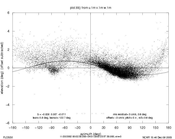
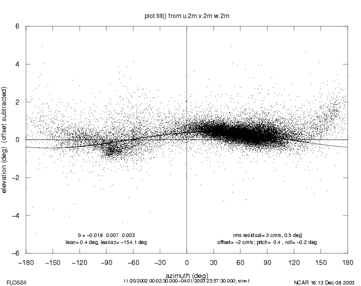
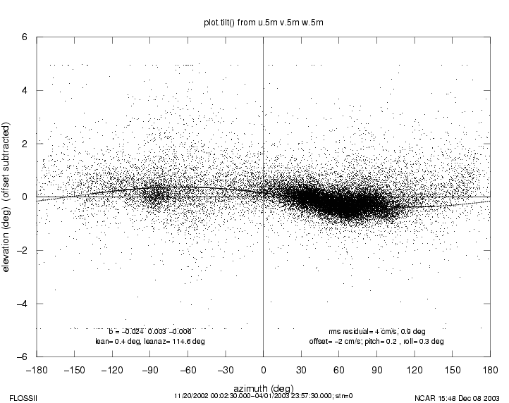
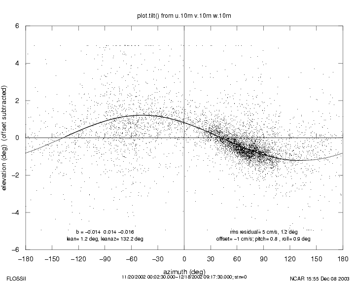
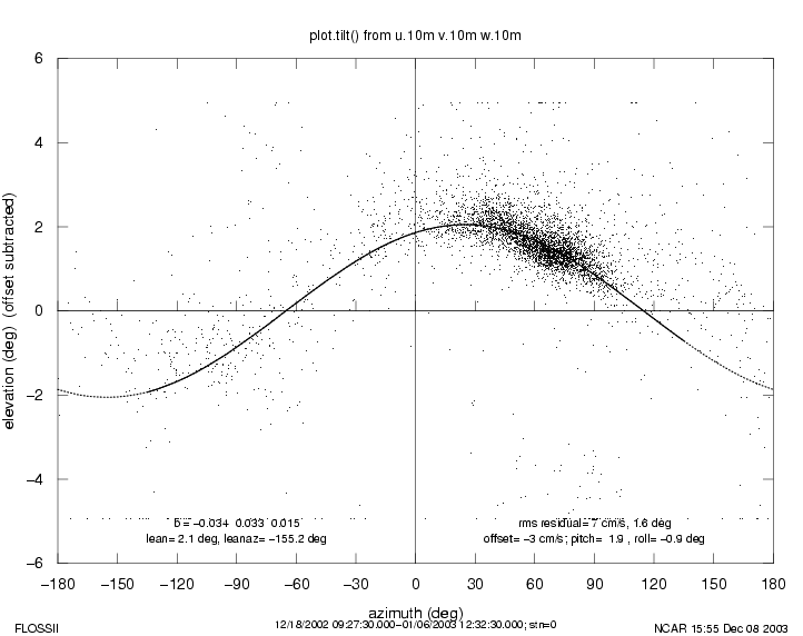
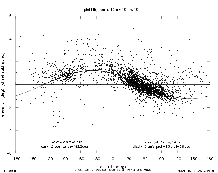
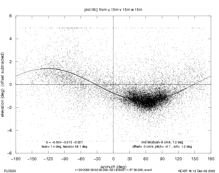
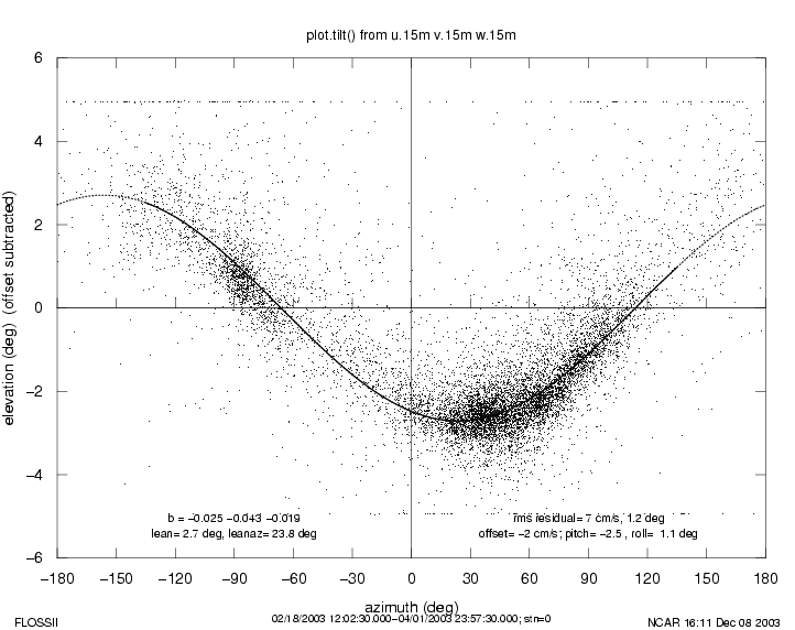
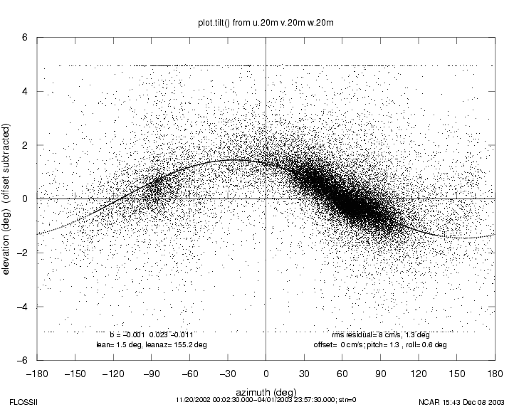
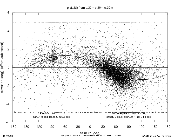
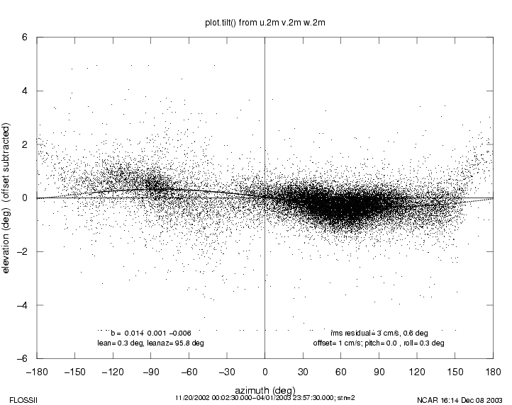
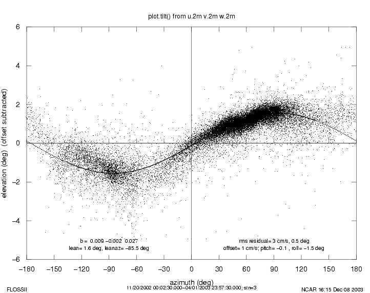
Sonic tilt angles have been evaluated using all the data.
| Sensor | w-bias (m/s) | Lean (deg) | LeanAz (deg) | Plot |
|---|---|---|---|---|
| 1m | -0.028 | 0.8 | 122.7 | plot |
| 2m | -0.018 | 0.4 | -154.1 | plot |
| 5m | -0.024 | 0.4 | 114.6 | plot |
| 10m: Before 18 Dec | -0.014 | 1.2 | 132.2 | plot |
| 10m: 18 Dec-6 Jan | -0.034 | 2.1 | -155.2 | plot |
| 10m: After 6 Jan | -0.034 | 1.2 | 142.2 | plot |
| 15m: Before 18 Feb | -0.004 | 1.4 | 58.1 | plot |
| 15m: After 18 Feb | -0.025 | 2.7 | 23.8 | plot |
| 20m | -0.001 | 1.5 | 155.2 | plot |
| 30m | 0.035 | 1.3 | 122.5 | plot |
| sage | 0.014 | 0.3 | 95.8 | plot |
| lake | 0.009 | 1.6 | -85.5 | plot |
We attempted to level all of these sensors during installation by using an electronic level to adjust (boom) guy wire tension and then attaching the anemometer. This should have been accurate to about 0.2 deg. Thus, we assume that these above "tilts" actually indicate real air motion due to local topography. Thus, none of these tilts have been removed from the data. If the user is interested in applying our rotation procedure, see our tilt correction page.
Here is a list of serial numbers:
2m	1389 (2.6cm)
10m	1391 (2.6cm)
20m	1392 (2.6cm) changed to 1390 (2.0cm) on 6 Jan
30m	1394 (2.6cm)
sage	1133 (1.2cm) changed to 1395 (2.6cm) on 18 Nov
lake	1393 (1.242cm) changed to 1397 (2.6cm) on 18 Nov
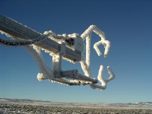
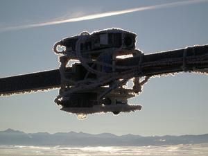
All kryptons had extensive periods of bad data, especially on cold (below -15C) nights. We now suspect that the cause of this is fog. To test the theory that this was due to frost build-up, we attached a hot-air blower to main.2m on 12/16 (not operational until 12/18), which helped a bit on 12/22-24, but not as much as expected. The pump on this blower seized up the next day. On the morning of 1/7, this problem recurred and was observed to be related to the presence of ice fog. Whether fog was always the reason is still unknown. (The fog on 1/7 was accompanied by extensive "feather" rime which was visible on the Axis camera images, but the camera didn't show this rime during other bad krypton events.) Tests of 3 kryptons (both head and electronics) in the lab showed normal operation down to -40 C, so this problem is not simply a failure from low temperatures.
We will have removed the majority of obviously bad data by using the criteria: |kh2o-H2O]>1.8 g/m3 or kh2oV<50mV. Some bad data will slip through this filter -- especially during the transitions between rimed and ice-free conditions.
Also, the 20m krypton showed a diurnal variation not seen by other kryptons. The onset appears to be related to incoming short-wave radiation, but this problem continues into darkness. We saw a hint of similar behavior in FLOSS01 that appeared to be caused by corrosion in the electronics box that was fixed during IHOP02. The 20m sensor was replaced on 1/6.
For the first time, we monitored pressure in the line close to the sample cell. It read about 10% lower than ambient pressure, a value which probably is typical of most of our deployments -- certainly FLOSS01. However, on 1/6 the inlet flow rate was changed from 6 to 7 lpm, which caused this pressure sensor to go offscale. We lowered the flow rate back to 6 on the next visit. During the period when it ran offscale, Plicor appeared to be approximately 82% of P, so we will synthesize a corrected Plicor from P at stn1 (itself a derived quantity that implements a correction for sensor temperature -- see "Barometer" below). (The top and bottom magenta lines in this plot show the uncorrected and corrected Plicor values.)
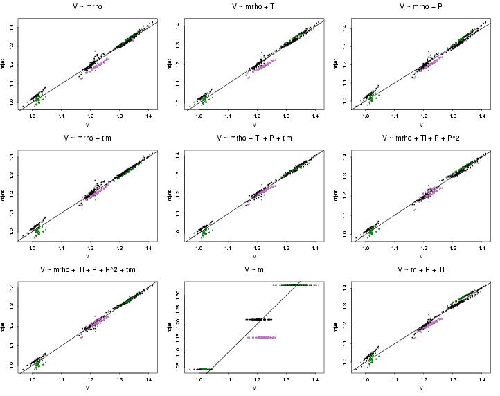
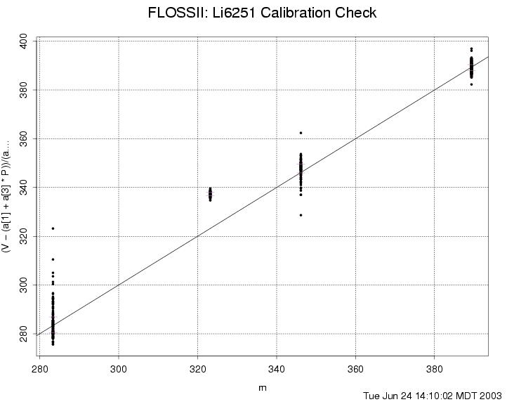
We have investigated data from the calibration periods and find that most of the data are well fit by voltage linearly related to CO2 density, computed using the calibration gas mixing ratio and the sample cell temperature and pressure (see plot). The data from the first 3 weeks (before the Hi-Cal regulator was installed) appear to have an offset from the rest of the data. Also, the Lo-Cal data at the end of the program are more scattered -- even from earlier data using the same Lo-Cal cylinder. The cause of both of these effects is as yet unknown. Thus, we have applied the regression from the middle 2 months (7 Jan - 21 Mar) to the entire period, noting that only the sensor gain is important for the flux measurements desired for FLOSS.
To obtain a slightly reduced residual, we added an extra term to the fit: V ~ a1 + a2*m*rho + a3*P. With this fit, we compute CO2 mixing ratios during the calibration periods. Our plot of the mixing ratios thus computed versus those of the cylinders shows that there still is a disturbing amount of scatter. However, the barely-discernable horizontal lines on this plot indicate that the first and third quartiles are generally within a range of +/-2 ppmV of the calibration cylinder values (except for those from the 323.26 ppmV cylinder used at the beginning).
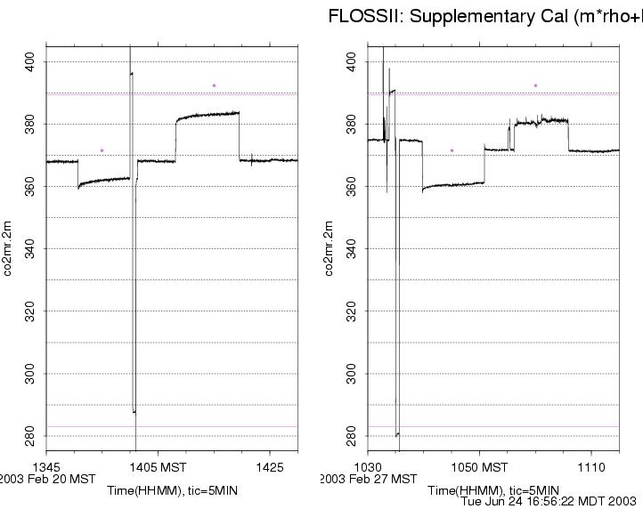
As a further check of these calibrations, we show data from "supplementary calibrations" done on 20 and 27 Feb. During these calibrations, gas from other CO2 calibration cylinders were introduced to the Li6251 at the inlet, rather than at the analyzer. Both of these calibrations were performed (on purpose?) at the time of automatic calibration cycles. A plot of these supplementary calibrations shows rather poor absolute values. (In this plot, the horizontal lines represent the value of the automatic calibration cylinders, the dots are the value of the supplementary calibration cylinder and indicate the supplementary calibration time, and the black line is the LiCor output calibrated using the fit described above.) The 20 Feb case shows that the above calibration produces values which are about 9ppmV lower than the supplementary cals but also about 5-7ppmV higher than the automatic cals. However, the 27 Feb case shows the supplementary cals now 12ppmV lower, with the automatic cals nearly matched. For such differences to exist between automatic and supplemental cals, there must be a response of our system to pressure or perhaps temperature variations that we have not characterized. (Even though the automatic cals themselves go through a wide range of pressures and temperatures.) Clearly, it will take more work to interpret the usefulness of these supplemental cals!
CO2 data have NOT yet been included in the final data.
Note also that these sensors ingested ice crystals during riming events (and possibly snow) -- see logbook, e.g., comments 169 and 173 and photos. No attempt will be made to eliminate these data.
There were several cases that fans were noted as not working (see below). During the days before these times, temperatures could be higher than ambient during the day and lower than ambient at night, due to radiative heat transfer -- especially in light winds. These cases sometimes are apparent in the temperature profiles or in comparisons with tc from a nearby sonic anemometer. We have filtered these data by removing data with |Tc(z)-tc(z)|>0.5C during the period when the fans were logged as having problems. (Tc is the acoustic virtual temperature computed from T, RH, and P.) Note that this is a pretty liberal criteria which probably retains some bad data, though it also could reject good data when the sonic data are bad.
Specific problems:
Roof-top test results:
ic_trh:
TestID	S/N	50Y		FLOSS Location	Roof:dT	Bath:dT	Roof:dRH Bath:dRH        Notes
				beg     end     degC    degC     %        %
a	001	T3510005	-	0.5	+0.059	+0.10	-1.6	-3.0		bell broken
b	206	R4910001	0.5	1	-REF-	+0.01	-REF-	 0.0		bell broken
c	104	T1140031	-	2	-0.006	+0.07	-1.0	-2.0		bell broken
d	701	T3510004	-	5	-0.112	-0.05	-1.2	-1.5		bell broken
e	702	T2620019	5	10	-0.060	-0.07	-0.1     0.0
f	007	T0820012	15	same	+0.011	+0.03v	-0.3    -0.5
g	704	09N001		20	same	+0.024	+0.00	-0.4	-1.5		new fan
h	008	U5020029	25	same	+0.051	 0.00	 0.0    -0.5
i	003	T1130007	30	same	-0.008	+0.03	+0.2     0.0
j	101	P1110024	sage	same	-		-			no inlet
k	502	R4910005	lake	same	-		-			no inlet
l	703	P1110027	1	-	+0.007	-0.02	-0.6    -0.5
m	004	U5020030	2	-	-0.012	 0.00	-2.3	-3.5		bell broken during tear-down
n	204	P4920040	10	-	-0.034	+0.01v	+1.0     0.0

ic_rad:
i	003	T1130007	30	same						bad until end
j	206	R4910001	0.5	1	-REF-	+0.01	-REF-    0.0
k	101	P1110024	sage	same	+0.015	+0.01	-0.2     0.0
l	502	R4910005	lake	same	-0.025	-0.01	-1.0    -1.5

-	005	P1110023	spare	spare	-	+0.01	-	-1.0
All upward-looking sensors were set up for forced ventillation, though it was discovered that electrical noise from the fans caused noise in the Tsoil measurements (same problem as in IHOP02). Thus, the fans were unplugged 12/4?-12/18 at Lake and Sage. (The fans were left on at the main tower site.) While they were unplugged, snow could (and did at least sometime) accumulate to cover the domes. This problem was "fixed" on 12/13-18 by both reprogramming the loggers to delay before sampling the Tsoil probes and by adding a capacitor in parallel with the fans to reduce the amount of electrical noise. After these fixes, Tsoil looked okay at Lake and Sage, though the tower sensors still show a slight amount of noise.
Net radiometers were used at all 3 sites. They were the only radiometers at Lake and Sage from 10/11 - 11/18. However, during this period, a logger program problem prevented data from being acquired until 11/18-19. All Rnet values should be normal (albeit, sometimes with ice cover) after then.
Upward and downward pyranometers were deployed at all 3 sites starting 11/18-20 using Kipp and Zonen radiometers. All appear to have operated normally.
Upward and downward pyrgeometers were deployed at all 3 sites starting 11/18-20 using Epply sensors. In addition, downward-looking pyrgeometers were deployed over two other surface types (mostly bare ground (12/17) and greasewood (1/7)) near the main tower to extend the lower sampling. An upward and a downward-looking sensor were mounted at 4m over this bare patch (also 12/17) as a second level in the flux-divergence array. A pair (for redundancy) of upward and downward-looking sensors were mounted at 25m (12/17, though trolley not extended until 12/18) as the third level of the flux divergence array.
Note that the "bare" site was approximately north of the main tower and thus was shaded by it from direct sun about noon every day. This wasn't considered a problem since the long-wave flux divergence sub-experiment only needs data at night.
All of these pyrgeometers were carefully calibrated in our oil bath, so that accuracies of <1 W/m2 could be obtained. However, Tdome-Tcase from the 25m and 4m.in.bare pyrgeometers were odd after setup. A wiring problem in the logger was discovered and fixed on 1/27. This cable swap also caused the wrong calibration coefficients to be applied to these signals. Our S-functions dat.Tdome and dat.Tcase have been changed to correct this problem. The 4m.in.bare "problem" appears to have corrected itself by January.
| Variable Name | Station | S/N | B * (lab) | B * (roof) | f(%) * (roof) | Notes |
|---|---|---|---|---|---|---|
| Rlw.in | 1 (grass site) | 26416 | 2.9 | 2.4 | 0.9 | |
| Rlw.in | 2 (sage) | 26417 | 2.6 | 2.1 | 1.3 | |
| Rlw.in | 3 (lake) | 29137 | 1.7 | - | - | Faulty case temperature (Tcase). Removed Dec 4. |
| Rlw.out | 1 (grass site) | 29260 | 3.4 | 2.9 | 1.1 | |
| Rlw.out | 2 (sage) | 27907 | 3.5 | 2.5 | 0.2 | |
| Rlw.out | 3 (lake) | 29136 | 2.3 | 1.8 | 1.9 | |
| Rlw.in.4m | 0 (bare site) | 31981 | 3.6 | 2.1 | 1.1 | Installed Dec 17 |
| Rlw.out.4m | 0 (bare site) | 31980 | 3.9 | 1.9 | 1.2 | Installed Dec 17 |
| Rlw.out.bare | 0 (bare) | 31976 | 3.0 | 2.5 | 0.5 | Installed Dec 17 |
| Rlw.out.grease | 0 (greasewood) | 31978 | 3.5 | 3.0 | 0.9 | Connected Jan 7 |
| Rlw.in.a.25m | 0 (tower) | 31975 | 2.9 | 2.4 | 0.7 | Installed Dec 17 |
| Rlw.in.b.25m | 0 (tower) | 31979 | 3.2 | 2.7 | 0.8 |
Installed Dec 17. Removed Jan 7, to check questionable case and dome temps. Reinstalled Jan 27, 15:30 MST |
| Rlw.out.a.25m | 0 (tower) | 31974 | 3.1 | 2.6 | 0.5 | Installed Dec 17. Removed Jan 7, to check questionable case and dome temps. Reinstalled Jan 27, 15:30 MST |
| Rlw.out.b.25m | 0 (tower) | 31977 | 2.4 | 1.9 | 1.2 | Installed Dec 17 |
* The above B and f values are used in the calculation of the long wave
radiation (Rlw) from the pyrgeometer thermopile value (Rpile) and the case and
dome temperatures:
Rlw = Rpile + SB * ( Tcase^4 + B * ( Tcase^4 - Tdome^4 ) ) + f * Rsw
At the end of the project, we ran a side-by-side comparison of all of the pyrgeometers on the roof of FLAB. During this comparison, we made a set of shading tests to evaluate the response to short-wave radiation. Several of the short-wave tests did not make sense (show an inverse top-hat response when shaded) using the above (laboratory-derived) B values. It was possible to obtain top-hat response for all sensors by making the B values smaller. However, using the set of B and f values thus obtained, there still are differences of up to 5 (typically 2) W/m2. (We note that even larger differences were seen during periods when the sensors weren't cleaned daily.) The QC-corrected data use the coefficients from the rooftop tests. We will leave any additional corrections to the user.
The soil temperature measurements were good, with the exception of the fan noise problem noted above in the radiometer section. Also, Tsoil.a.2.5cm at Sage had extreme variations. This could have been due to the sensor being exposed to air. However, subplot "a" was directly underneath a sage bush, so the dirt around this sensor could have been heated by the plant material (which is black). We decided to leave this sensor alone and its data have been retained in the final data set.
The soil heat flux probes were mostly okay, with the following notes:
The soil moisture probes (Ech2o) all reported values, with the following notes:
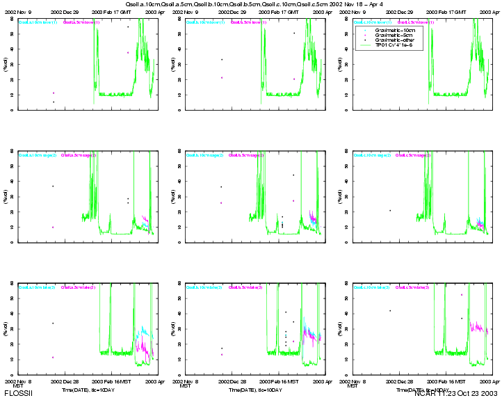
However, an e-mail exchange that we had with the manufacturer after the project explained that these probes (and others that depend on the electrical properties of the soil, including our CS615 and TRIME probes) do not detect frozen water. Thus, MOST OF OUR SOIL MOISTURE MEASUREMENTS ARE NOT VALID. The data have been edited to remove all Qsoil measurements when the corresponding Tsoil is below zero. This removes all but the last few weeks (spring thaw) of data at the Sage and Lake sites. (The grass cover at Grass insulated the soil so it remained frozen through the end of the project.) We made a few gravimetric measurements at each subplot which also should be valid. A plot shows all of the good soil moisture measurements. In this plot, rows correspond to the grass, sage, and lake sites (from top to bottom) and subplots a, b, and c (left to right); Ech2o measurements are lines (blue=10cm; magenta=5cm) and gravimetric samples are dots, colored to correspond to the Ech2o locations when appropriate. Obviously, not much data remain. It should be possible to correlate the TP01 heat capacity values (see below) with soil moisture, though these measurements were not made in the same subplots. (The TP01 values are shown in the above plot as green lines.) This task will be left to the user.
In addition, we deployed a soil thermal property probe (Hukseflux TP01) at each site. This is a new measurement for ISFF, but should provide a better estimate of soil heat capacity than we have made for earlier studies (using mass-weighted bulk thermal properties and crude estimates of soil composition). Also, these probes measure the soil thermal conductivity, which is needed to correct our soil heat flux measurements. Unfortunately, we did not obtain these probes until the soil was frozen and we also had some wiring errors (though little data were lost because of the wiring since the probes took a long time to settle). Thus, a complete data set is not available until 1/27. It appears that these probes needed to settle in the frozen ground -- they were installed with a slight (<1mm) air gap with the soil. The data appear to show that none of the probes were really settled until a soil warming period at the end of January (see plot). Additionally, the signals from the probes at lake and sage had significant noise, caused by the voltage controller of the PAM station. We fixed this noise with a voltage regulator on 2/22, though the data before appear to usable.
The snow depth gauge was noisy since it was deployed, similiar to its behavior during FLOSS01. Thus, the data probably are useless, even though the mean value is nearly correct. We moved it on 1/6 to a location which shouldn't see interference from the radiometer stand legs, but the noise didn't change. Nevertheless, these data are included in the final data set since they appear to be a reasonable indication of when it was snowing (when the signal has large variations and often goes to zero)!
As mentioned above, the krypton hygrometers appear to be a good indicator of fog!
FLOSS2 Field Logbook
A computer-readable field logbook
of comments noted by NCAR and other personnel is available in read-only
html form and updated every day.
| Oct 1, 2002 | Nov 20, 2002 | Nov 21, 2002 | Dec 4, 2002 | Jan 27, 2003 | IOP: Feb 17 - Mar 7 |
| Ice Detectors |
| Oct 10, 2002 | Nov 20, 2002 | Jan 7, 2003 | Jan 27, 2003 | IOP: Feb 17 - Mar 7 | TCAM test: Mar 26-27 |
| Oct 10, 2002 | Nov 20, 2002 | Dec 4, 2002 | Jan 27, 2003 | IOP: Feb 17 - Mar 7 |
| Univ. of Wyoming KingAir | Wildlife | Misc |
Note that the exposures of these images vary considerably -- even between the 15-minute shots. We highly recommend examining the entire set of images for any serious use of these images.
Daily QC Plots
Preliminary time series, profile and spectra plots
are available for review of data quality.
The time series plots are of the 5-minute statistics, covering 48 hours,
centered on local noon of each day. Hourly profiles from the 30 meter tower
are plotted from 5-minute or 30-minute means, as labeled.
Spectra plots are made from 30-minute periods of high-rate sensor data,
starting at the stated time.